Placed-based approaches to addressing disadvantage
Linking science and policy
You are in an archived section of the AIFS website
There is mounting evidence that the rapid social and economic changes associated with globalisation, economic restructuring and demographic change have had differential impacts (both positive and negative) across Australia's cities and towns (Gregory & Hunter, 1995; O'Connor, Stimson & Taylor, 1998; Stimson, 2001). Gregory and Hunter provided a stark account of growing inequality across Australian neighbourhoods. Their study showed that while population averages can show a general pattern of improvement, this can hide vastly different experiences across neighbourhoods of different socio-economic status.
Notwithstanding a period of prolonged economic growth (preceding the global financial crisis), more recent research indicates that disadvantage is becoming increasingly concentrated in some locations, reinforcing spatial inequality. Indeed, Stimson (2001) observed that despite strong national economic performance, the disparity across areas seems likely to get worse. Vinson (2007) found that a relatively small number of localities accounted for a much greater share of disadvantage across a wide range of indicators, including unemployment, low income, criminal convictions, child maltreatment and early school-leaving. Similarly, Baum (2008) stated that while disadvantage has been a feature of Australian cities for some time, current forms of place-based disadvantaged have become more entrenched and more difficult to escape.
Government agencies, both Commonwealth and state, deliver a broad range of programs to improve the economic, social and community wellbeing of Australians. Traditionally, many of these policies and programs have focused on single aspects of socio-economic disadvantage at a national or state level; that is, they aim to provide universal support to people who experience a particular form of disadvantage. Wolff and de-Shalit (2007) described this approach as one based on sectoral justice, where different aspects of disadvantage are considered independently, often demarcated along lines of portfolio responsibilities.
As evidence and concern about the spatial concentration of disadvantage has accumulated, a range of place-based policy responses have emerged across different levels of government. There is a long history of debate around the relative merits of place-based versus the more mainstream people-based policies for addressing disadvantage (see, for example, Winnick, 1966, and, more recently, Griggs, Whitworth, Walker, McLennan, & Noble, 2008). In their recent review, Griggs et al. argued that:
the reality, of course, is that all people live in places, contribute to places and are affected by places. Poverty and disadvantage are mediated by place, and places are affected by the poverty or otherwise of their inhabitants. Hence, it is reasonable to suspect that policies that dissociate people from places and vice versa may perform poorly. (p. 1)
Griggs et al. (2008) also provided a useful discussion of the distinction between people and place policies that went beyond a simple dichotomy, but rather used a matrix based on the major focus of the policy and the intended impact. This matrix resulted in four different types of policies: place-focused to affect place, place-focused to affect people, people-focused to affect people, and people-focused to affect place. While this matrix provided a useful way to help evaluate different policies, ultimately Griggs et al. identified the need for increasing recognition of holistic person and place approaches. Similarly, Randolph (2004) considered that the distinction between people- and place-based approaches is often somewhat artificial, as the ultimate aim for the vast majority of place-based programs is to improve outcomes for people. Baum, Stimson, O'Connor, Mullins, and Davis (1999) concluded that a mixed person-place focus is needed that uses actions in some places to enable their inhabitants' participation, but does not need to be applied in all places.
Arguably one of the strongest justifications supporting place-based approaches is that they enable the targeting of people experiencing multiple and inter-related forms of disadvantage and provide a platform for the delivery of a more integrated and holistic suite of services and supports. Far from being viewed as a replacement for mainstream approaches, they are widely considered to provide a complementary form of support that can be used where the breadth and complexity of disadvantageous factors may limit people's ability to benefit from mainstream services and supports. Indeed, the overall success of place-based programs is largely considered to be contingent on the extent to which targeted place-based polices and mainstream people-based services and support are integrated and mutually reinforcing (Beer & Forster, 2002; Griggs et al., 2008; Randolph, 2004; Smith, 1999).
Nevertheless, it is important to note that the use of a place-based approach does not necessarily automatically mean better coordination and integration across different spheres of social policy. In a case study of place-based initiatives in Western Sydney, Randolph (2004) identified some 36 separate programs spanning 13 different government departments, with many using different methods of spatial targeting. To an extent, this reflects the relatively recent emergence of place-based approaches and the lack of a coherent overarching framework to guide their implementation.
There are some very practical questions to explore as we move from problem identification to a policy design and implementation phase. This paper will explore two such questions that could have quite important implications for shaping place-based policy responses. Firstly, what is the impact of scale on identifying place-based disadvantage and, secondly, how can we account for the potential impact of population mobility when trying to understand the outcomes of place-based approaches?
Methods
The impact of scale on identifying place-based disadvantage
The approach adopted in this analysis was to explore the extent to which small areas of concentrated disadvantage are nested within a range of larger spatial units and how this correspondence varies across different levels of disadvantage, by state and territory, and by remoteness area classification.
The underlying assumption being tested is that smaller areas of concentrated disadvantage will be located within and therefore still broadly identified by analysis across larger areas. Put more simply, the approach asks how much the unit of analysis alters the identification of concentrated disadvantage.
The data used for this analysis is from the 2006 Australian Bureau of Statistics (ABS) Socio-Economic Indexes for Areas (SEIFA) Index of Relative Socio-Economic Disadvantage. While there are numerous different measures of disadvantage available, the SEIFA Index of Relative Socio-Economic Disadvantage was considered highly suitable for this investigation because it is widely used, covers numerous different dimensions of disadvantage, and is available at a range of spatial scales.
Before exploring the impact of aggregating results across different geographies, results from a test of global spatial autocorrelation based on the smallest spatial unit available are presented. This analysis used the Moran's I with an inverse distance weighting (no threshold value was used). Global measures of spatial autocorrelation such as
Moran's I provide an indication of the extent to which areas that are closer to one another share more in common than areas that are further away. Scores range from 1 (which indicates complete clustering) to -1 (which indicates complete dispersal), while a score of 0 indicates a random distribution. The probability, or p value, indicates the extent to which the observed score could have occurred purely by chance.
The paper then uses four different levels of disadvantage - representing the most disadvantaged 10%, 5%, 2% and 1% of localities across four different spatial units - to explore the extent to which smaller areas of disadvantage were nested within and thereby still covered by analysis across larger areas. A geographic information system (GIS) was used to explore the extent of overlap between areas identified based on the different units of analysis. The spatial scales used in this analysis are:
- Collection District (CD) - CDs are an ABS boundary and represent the smallest units for which most Census data are available (representing an area of approximately 220 households). In 2006, there were a total of 37,457 CDs for which a SEIFA score was available.
- State Suburb (SSC; excluding unclassified areas) - SSCs are an ABS boundary that are derived by using whole CDs to make a best fit to gazetted suburb boundaries. The SSC unit used in this analysis does not include any unclassified areas (i.e., those not covered by a gazetted suburb boundary, most notably remote parts of Northern Territory) and therefore does not cover all of Australia. In 2006, there were 8,267 SSCs with a SEIFA score.
- Postal Area (POA) - POAs are an ABS boundary that assigns postcodes to each CD. Where a CD covers more than one postcode the CD is assigned to the postcode that contains the highest proportion of the population. In 2006, there were 2,478 POAs with a SEIFA score.
- Statistical Local Area (SLA) - SLAs are an ABS boundary that are based on the aggregation of one or more whole CDs. In 2006, there were a total of 1,395 SLAs with a SEIFA score.
In addition to these units, the Remoteness Area (RA) classification was used to identify whether a CD was located in a major city, inner regional, outer regional, remote or very remote area (ABS, 2006).
Exploring population mobility and place-based disadvantage
Accepting the view that, ultimately, any place-based approach needs to translate into better outcomes for people, there is a clear need to understand the dynamic nature between people and place. Drawing on detailed information from a series of in-depth case studies, Fincher and Wulff (2001) noted the complex way in which both short-term and longer term mobility interacts with the material conditions experienced by people, both in terms of those who move and those who remain in communities with high mobility. Although recent research confirms the existence of spatial disparities, Fincher and Wulff also concluded that places with concentrations of disadvantage are changing. Understanding patterns of mobility across areas of concentrated disadvantage is a small but potentially important step towards disentangling the relationship between changes at the person and area level.
This paper draws on data from the 2006 ABS Census of Population and Housing to explore the link between population mobility and disadvantage, as measured by the 2006 SEIFA Index of Relative Socio-Economic Disadvantage.
The 2006 Census included a series of data relating to peoples' place of residence five years ago. These data are used to calculate the proportion of the population of each CD falling into the following groups:
- those living at the same address in 2006 as five years ago;
- those living at a different address in the same SLA five years ago;
- those living at a different address in a different SLA five years ago;
- those living at a different address overseas five years ago;
- those living at a different unspecified address five years ago; and
- those whose previous address was not stated.
Data on population movement are then compared to CD scores on the SEIFA Index of Relative Socio-Economic Disadvantage.
Discussion of findings
Does scale matter?
There is a relatively large body of research exploring different indicators for identifying locations of concentrated disadvantage. In contrast, there is comparatively little investigation of how the scale or geographic unit used will affect the areas identified. Often, decisions about geographic scale are at least partly determined by the availability of data for the preferred indicators. This paper is not arguing that ensuring indicators have a sound theoretical basis is unimportant, because this is clearly a key concern for any good measure. Rather, this paper aims to explore how much impact the scale of analysis can have on the identification of disadvantaged areas over and above the choice of specific indicators used.
Results from the global test of spatial autocorrelation indicate that there is a statistically significant clustering of SEIFA scores across CDs (Moran's I = 0.14, Z = 675.35, p < .01). While this partly supports the view that it is sensible to scale up and aggregate these smaller units, the value of Moran's I suggests that, while present, the degree of clustering is limited.
Table 1 shows for each state and territory the proportion of the most disadvantaged CDs based on the SEIFA Index of Relative Socio-Economic Disadvantage that were located within the most disadvantaged areas identified across larger spatial scales. The "Total" row for each level of disadvantage represents the share of disadvantaged CDs in each state and territory (for example, New South Wales contained just under 36% of the most disadvantaged 10% of CDs). The "Total" column represents the figure for Australia as a whole (for example, only just over 24% of the most disadvantaged 10% of CDs across Australia were located in the most disadvantaged 10% of SLAs). The degree of overlap between disadvantaged CDs and larger spatial units tends to decrease as the focus shifts to more extreme levels of disadvantage. While smaller geographic units tend to show higher correspondence with the location of disadvantaged CDs, only just over half of the most disadvantaged 10% of CDs were located within the most disadvantaged 10% of SSCs. It is interesting to note that POAs show much less variation in the proportion of CDs within larger units across the different levels of disadvantage. However, this is largely a result of alignment across remote and very remote areas, which offers limited spatial accuracy (as seen in Table 2).
| NSW (%) | VIC (%) | QLD (%) | SA (%) | WA (%) | TAS (%) | NT (%) | ACT (%) | Total (%) | |
|---|---|---|---|---|---|---|---|---|---|
| Most disadvantaged 10% | |||||||||
| SLA | 12.8 | 23.6 | 28.2 | 43.9 | 23.5 | 11.2 | 83.3 | 30.0 | 24.1 |
| POA | 35.1 | 46.0 | 29.3 | 58.6 | 38.6 | 48.9 | 75.9 | 0.0 | 41.0 |
| SSC | 56.7 | 57.2 | 54.0 | 67.5 | 66.1 | 76.4 | 5.6 | 30.0 | 57.7 |
| Total | 35.7 | 19.2 | 16.8 | 11.7 | 8.5 | 4.8 | 2.9 | 0.3 | |
| Most disadvantaged 5% | |||||||||
| SLA | 0.0 | 0.0 | 12.6 | 4.3 | 17.2 | 0.0 | 71.9 | 0.0 | 7.6 |
| POA | 27.4 | 30.5 | 38.7 | 48.0 | 44.4 | 44.3 | 79.2 | 0.0 | 37.4 |
| SSC | 46.9 | 46.9 | 55.2 | 60.9 | 64.5 | 62.0 | 0.0 | 0.0 | 49.7 |
| Total | 36.0 | 16.3 | 13.9 | 14.9 | 9.0 | 4.2 | 5.1 | 0.3 | |
| Most disadvantaged 2% | |||||||||
| SLA | 0.0 | 0.0 | 0.0 | 0.0 | 6.4 | 17.0 | 14.7 | 44.0 | 11.9 |
| POA | 74.7 | 12.1 | 41.1 | 43.9 | 0.0 | 63.4 | 75.2 | 0.0 | 35.7 |
| SSC | 12.5 | 71.9 | 77.4 | 76.2 | 0.0 | 0.0 | 20.2 | 35.5 | 40.9 |
| Total | 33.1 | 12.6 | 10.0 | 14.3 | 13.5 | 4.3 | 11.2 | 0.5 | |
| Most disadvantaged 1% | |||||||||
| SLA | 0.0 | 0.0 | 0.0 | 0.0 | 0.0 | 0.0 | 5.3 | 52.6 | 9.9 |
| POA | 89.5 | 0.0 | 29.0 | 16.1 | 0.0 | 62.5 | 77.5 | 0.0 | 38.9 |
| SSC | 0.0 | 33.3 | 47.9 | 76.7 | 0.0 | 0.0 | 9.7 | 19.4 | 32.8 |
| Total | 24.8 | 11.5 | 10.1 | 8.3 | 21.3 | 3.2 | 19.5 | 0.5 | |
Source: ABS Census of Population and Housing, 2006
It is also important to note that the results vary considerably across different states and territories. New South Wales has the highest share of disadvantaged CDs across each level of disadvantage investigated, yet at the same time it has among the lowest level of correspondence across the various geographic units. Perhaps the clearest indication is that none of the most disadvantaged 5%, 2% or 1% of CDs in New South Wales are located within the SLAs of the same level of disadvantage. Again, the smaller geographic units tended to exhibit a larger degree of correspondence, but even the most disadvantaged 10% of SSCs in New South Wales contained only just over half of the most disadvantaged 10% of CDs. As expected, the overall share of the most disadvantaged CDs located in Western Australia and the Northern Territory increased at the more disadvantaged end of the spectrum, reflecting the fact that many of the most disadvantaged CDs are located in remote Indigenous communities.
Data in Table 2 is based on the same approach as in Table 1, but has been disaggregated by Remoteness Area classifications instead of by state and territory. As was the case previously, column totals represent the figure for Australia as a whole and row totals represent the share of disadvantaged CDs within each Remoteness Area classification. This analysis also demonstrates that the degree of alignment varies widely based on different Remoteness Area classifications. Major cities accounted for the highest proportion of disadvantaged CDs, with the exception of the most disadvantaged 1%. Just under half of the most disadvantaged 1% of CDs occurred in very remote areas. Only very remote areas had more than 50% alignment between the most disadvantaged CDs across each of the other geographic units and levels of disadvantage. By contrast, disadvantaged CDs in inner regional locations rarely were located within similarly disadvantaged larger areas. None of the most disadvantaged 5%, 2% or 1% of CDs in major cities occurred within SLAs identified based on the same proportional thresholds.
| Major cities (%) | Inner regional (%) | Outer regional (%) | Remote (%) | Very remote (%) | Total (%) | |
|---|---|---|---|---|---|---|
| Most disadvantaged 10% | ||||||
| SLA | 26.3 | 5.9 | 14.3 | 35.7 | 81.6 | 24.1 |
| POA | 47.7 | 15.3 | 30.8 | 49.2 | 90.1 | 41.0 |
| SSC | 61.9 | 47.6 | 55.8 | 61.9 | 60.9 | 57.7 |
| Total | 52.0 | 21.3 | 16.5 | 3.4 | 6.8 | |
| Most disadvantaged 5% | ||||||
| SLA | 0.0 | 0.3 | 0.9 | 17.6 | 55.9 | 7.6 |
| POA | 38.5 | 11.5 | 19.8 | 41.9 | 85.9 | 37.4 |
| SSC | 52.9 | 32.8 | 49.6 | 52.7 | 58.6 | 49.7 |
| Total | 54.3 | 17.2 | 12.4 | 4.0 | 12.1 | |
| Most disadvantaged 2% | ||||||
| SLA | 0.0 | 1.0 | 2.1 | 33.3 | 36.2 | 11.9 |
| POA | 21.5 | 4.2 | 12.8 | 30.6 | 81.2 | 35.7 |
| SSC | 39.9 | 24.0 | 34.0 | 30.6 | 53.6 | 40.9 |
| Total | 48.5 | 12.8 | 6.3 | 4.8 | 27.6 | |
| Most disadvantaged 1% | ||||||
| SLA | 0.0 | 0.0 | 7.7 | 17.4 | 18.2 | 9.9 |
| POA | 6.9 | 0.0 | 0.0 | 30.4 | 73.9 | 38.9 |
| SSC | 13.1 | 15.2 | 30.8 | 30.4 | 51.1 | 32.8 |
| Total | 34.7 | 8.8 | 3.5 | 6.1 | 46.9 | |
Source: ABS Census of Population and Housing, 2006
Previous research by Hunter (1996) indicated that there is a strong association between concentrations of socio-economic disadvantage and public housing, finding that 60% of the population in the most disadvantaged 5% of CDs in 1991 lived in public housing. This raises the question about the degree to which the concentration of disadvantage is purely as a result of the location of public housing. While the ABS 2006 Census of Population and Housing did not identify the number of individuals living in public housing across CDs, it did provide the proportion of dwellings in each CD that are public housing. Table 3 shows for each level of the most disadvantaged CDs the proportion of dwellings that were public housing (that is, those rented from a state or territory housing authority). While the proportion of public housing is much higher when focusing on the more disadvantaged CDs, even among the most disadvantaged 1% of CDs, only just over half of all dwellings were public housing. This suggests that while it is a factor (as you would expect given that public housing is a component of the SEIFA index), the concentration of disadvantage across small areas reflects a wider range of factors than just the concentration of public housing.
| Total number of dwellings | Dwellings that were public housing (%) | |
|---|---|---|
| Most disadvantaged 10% | 678,871 | 20 |
| Most disadvantaged 5% | 321,982 | 30 |
| Most disadvantaged 2% | 108,294 | 45 |
| Most disadvantaged 1% | 41,408 | 55 |
Source: ABS Census of Population and Housing, 2006
Even when using identical sources, clearly the scale at which data are analysed has important impacts on the identification of place-based disadvantage. Population characteristics have limited spatial homogeneity and larger geographic units tend to average out differences that are observable at smaller scales. These effects appear to become more pronounced as the level of disadvantage increases. Furthermore, there are significant differences in the extent of correspondence between different states and territories and across different Remoteness Area classifications.
The findings outlined in this paper are a very clear and practical example of what geographers call the modifiable areal unit problem (MAUP; see, for example, Openshaw, 1984). MAUP is a potential source of error that can affect spatial studies using aggregate data, where variation in scale causes variation in statistical results. Openshaw and Taylor (1979) highlighted that using the same data at different levels of aggregation could even change the sign of the coefficient describing the relationship between two variables. While relatively well understood by geographers, the MAUP has very significant implications for many areas of social policy that have largely been unexplored.
As was very briefly outlined earlier in this article, there is now compelling evidence of spatial inequality in a wide range of socio-economic outcomes, along with an increasing focus on the potential of place-based policy responses to address them. However, the ability of policy-makers to consolidate this research into a detailed understanding that can shape decisions about where to prioritise resources for place-based responses is complicated by issues of scale.The critical issue then becomes one of "fit for purpose"; that is, establishing at what scale place-based responses can most effectively work and what data are available to help identify places at this scale. Clearly, if responses that focus in on specific suburbs or even parts of suburbs are likely to be required, analysis of data at the SLA level, no matter how relevant, is problematic. At the core of this issue is the need to develop closer working relationships between science and policy.
What would improvement look like?
Despite the complexities outlined above, in many respects identifying locations of concentrated disadvantage at a point in time is a simpler task than establishing what constitutes improvement. On the surface, it seems reasonable to suggest that improvement be gauged by either changes in key statistics or the extent to which a location continues to show a concentration of disadvantage.
While both of these measures can be useful, in addition to the issues of scale, they are complicated by the relatively high rate of population mobility across the country. At the time of the 2006 Census, just over 40% of the population of people over the age of 5 years lived at a different address from where they lived in 2001 (ABS, 2009). In effect, this means that when examining change over time in some geographic locations, the data could relate to a very different group of people.
Figure 1 indicates that the proportion of the population who lived at the same address 5 years ago shows very little variation across SEIFA deciles (where the lowest SEIFA scores, the first decile, represent the most disadvantaged localities and the highest SEIFA scores, the tenth decile, represent the least disadvantage localities). While the overall rate of mobility changed little with increasing disadvantage, the nature of mobility was slightly different, with people in disadvantaged areas more likely to have moved within the same SLA and subsequently less likely to have moved from a different SLA or from overseas. It is also important to note that Fincher and Wulff (2001) highlighted that the Census data can significantly undercount population mobility, particularly for some disadvantaged groups such as low-income families and sole parents, who often move multiple times over a 5-year period.
Figure 1: Population mobility, by levels of disadvantage
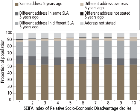
Source: ABS Census of Population and Housing, 2006
Where the ultimate goal of adopting a place-based approach is to improve outcomes for people, it is crucial to understand more about how many people have moved out of or into a location and the reasons why. At the most extreme level, improvement in area level statistics could be achieved simply by rearranging the population, without necessarily improving outcomes for any particular individual or family.
For example, consider a locality that contained a population of 2,000 people in 2001 that were considered highly disadvantaged. By 2006, a large housing development was built in the locality that saw an additional 2,000 individuals who were more advantaged move into the area. In this case, 2006 area level statistics would appear to improve, even if circumstances had not improved for any of the highly disadvantaged individuals or families. So despite this apparent improvement, the extent to which this represented a positive outcome in terms of enhancing social inclusion for the most disadvantaged people and families in that locality is questionable.
On the other hand, consider a location that had a population of 4,000 highly disadvantaged individuals in 2001. If in 2006 this area still had 4,000 highly disadvantaged individuals, it would be easy to conclude that no improvement had occurred. If a place-based program had been operating in this area, it would be tempting to say it had had no measurable impact on people in that location. Yet consider what this might mean if data showed that only 50% of the population in 2006 lived in the same suburb in 2001. Without knowing the outcomes for those that moved, it would be very difficult to determine if the program was making a difference. Indeed, it could be that people moved out of the area to pursue new opportunities and the subsequent availability of low-cost private or public housing meant a new group of highly disadvantaged people moved in. In this instance, mobility into and out of the location could mask any potential positive impact at the individual level. Even if this was the case for a proportion of those that moved, a very different conclusion about progress is likely.
In their recent evaluation of the Communities for Children place-based program, Edwards et al. (2009) used a series of longitudinal surveys and control sites to explore the impact of the program on people living in target communities (which represents one of very few Australian evaluations of place-based approaches to involve detailed longitudinal studies and control sites). While the study by Edwards et al. was able to identify people who had moved into different communities, the report did not explore where they moved to, the reasons for moving and if the people who moved had different outcomes. Research in the United States has focused much more explicitly on attempting to determine the extent to which mobility can help influence improved outcomes for people. Coulton, Theodos and Turner (2009) reviewed a decade-long program that aimed to improve outcomes for families by strengthening connections across their community. As part of this study, they explored the link between family mobility and neighbourhood change, finding that neighbourhood change is indeed often the result of mobility and the differences between the people who stay and those who move.
The United States has also trialled a large-scale experiment, called Moving to Opportunity, based on encouraging low-income households to move into lower poverty neighbourhoods (Orr et al., 2003). The Moving to Opportunity study was successful in promoting mobility to lower poverty neighbourhoods, at least in the short term. However, the extent to which these changes linked to long-term changes in individual circumstances appears mixed. Some small but important changes were reported in terms of health and education, but no changes to employment, wealth or receipt of public assistance were observed through the interim evaluation. Part of the explanation for these mixed findings appears to be the fact that often the move to locations of lower poverty was only temporary, with people either moving to an area where poverty was becoming increasingly more concentrated or making subsequent moves back to areas of higher poverty (Orr et al., 2003). The decision to move back to areas of higher poverty was found to be influenced by a range of factors, including family ties and difficulties with the housing market (Comey, de Souza Briggs, & Weismann 2008). While demonstrating that neighbourhoods can play a role in the transmission of social and economic status, Sharkey (2009) concluded that moving families may not be the most effective way of tackling concentrated disadvantage; rather, he advocated investing in disadvantaged neighbourhoods in ways that reduce the concentration of disadvantage and provide lasting economic benefits.
In their review of neighbourhood effects, Samson, Morenoff, and Gannon-Rowley (2002) concluded that research needs to better understand the interplay between neighbourhood selection decisions, structural context and social interactions. This observation rings particularly true in Australia, where very few, if any, examples of such research exist.
Three key questions can help guide a more detailed approach to understanding the impact of any locational approaches, namely:
- To what extent is concentrated disadvantage present in the same locations over time?
- To what extent are the same people present in these locations over time?
- What do we know about the characteristics of people who move into, out of, or stay in disadvantaged locations?
In essence, these questions amount to trying to disentangle the links between outcomes at the person level and those at the area level.
Conclusion
Through a series of simple analyses, this paper has attempted to draw out some key challenges related to linking evidence of concentrated disadvantage with targeted policy responses. While there is often considerable attention and debate around the various indicators of disadvantage, there is far less attention paid to ensuring that the geographic scale of analysis is directly related to potential options for targeted place-based approaches. This paper has clearly outlined the importance of scale by demonstrating that, even when using the same data, analysis based on different geographic units will identify quite different locations of disadvantage. Even analysis undertaken in very small areas, such as suburbs, can mask some highly localised areas of concentrated disadvantage.
The purpose of this paper has not been to suggest the "best" scale, but rather has aimed to demonstrate the importance of considering how well the scale of analysis fits with the intended response. Efficient and effective delivery of place-based responses will need to ensure that the evidence base used to identify priority areas be closely aligned with the scale of potential responses. Furthermore, different processes used to identify priority locations, based on different data at different spatial scales, will not necessarily identify the same locations and could thereby undermine the potential of place-based approaches to provide a more integrated and coordinated approach to service delivery. Put simply, a coordinated approach to working in locations of concentrated disadvantage needs to begin with a coordinated approach to identifying these locations.
While there are clearly some important implications for identifying areas of concentrated disadvantage, this paper has also highlighted a number of limitations in identifying and measuring changes that could result from place-based approaches. Australia has a relatively high rate of population mobility that poses a number of significant dilemmas for understanding the dynamic relationship between people and places. Place is increasingly being acknowledged as an important way of targeting disadvantage; however, the extent to which improvement can and should be gauged by improvement in area level statistics is questionable. Given the high rate of mobility, even across highly disadvantaged locations, any comparison of area level statistics over time are likely to, at least in part, be comparing outcomes for a different group of people.
Currently there is very limited information that enables the examination of longitudinal patterns of people moving into, out of, or staying in areas of concentrated disadvantage and the links between outcomes at the individual and area level. The ABS has recently trialled linking data across different Census collections, using a 5% sample from the 2006 Census. This project has considerable potential to help improve longitudinal data if it is included as part of future Censuses. Nevertheless, the extent to which any geographic analysis would be possible using the new dataset is unclear, but likely to be limited.
As evidenced by the strong spatial patterning of socio-economic disadvantage, place-based approaches have clear potential to help improve outcomes for people experiencing multiple and inter-related forms of disadvantage. Notwithstanding this potential, this paper has highlighted some important challenges related to targeting and monitoring place-based approaches. Addressing these challenges is the unique domain of neither scientific inquiry or policy formulation, but lies at the interface between science and policy. Forging these closer working relationships between science and policy is vital to achieving effective responses.
References
- Australian Bureau of Statistics. (2006). Statistical geography: Vol. 1. Australian standard geographical classification (ASCG), July 2006 (Cat. No. 1216.0). Canberra: ABS.
- Australian Bureau of Statistics. (2009). Migration Australia, 2007-08 (Cat. No. 3412.0). Canberra: ABS.
- Beer, A., & Forster, C. (2002). Global restructuring, the welfare state and urban programmes: Federal policies and inequality within Australian cities. European Planning Studies, 10(1), 7-25.
- Baum, S. (2008). Suburban scars: Australian cities and socio-economic deprivation (Urban Research Program, Research Paper 15). Brisbane: Griffith University.
- Baum, S., Stimson, R., O'Connor, K., Mullins, P., & Davis, R. (1999). Community opportunity and vulnerability in Australia's cities and towns. Brisbane: Australian Housing and Urban Research Institute.
- Comey, J., de Souza Briggs, X., & Weismann, G. (2008). Struggling to stay out of high poverty neighbourhoods: Lessons from the Moving to Opportunity experiment (Brief No. 6). Washington, DC: Urban Institute.
- Coulton, C., Theodos, B., & Turner, M.A. (2009). Family mobility and neighbourhood change: New evidence and implications for community initiatives. Washington, DC: Urban Institute.
- Edwards, B., Wise, S., Gray, M., Hayes, A., Katz, I., Mission, S. et al. (2009). Stronger families in Australia study: The impact of Communities for Children (Occasional Paper No. 25). Canberra: Department of Families, Housing, Community Services and Indigenous Affairs.
- Fincher, R., & Wulff, M. (2001). Moving in and out of disadvantage: Population mobility and Australian places. In R. Fincher & P. Saunders (Eds.), Creating unequal futures (pp. 158-194). Crows Nest, NSW: Allen & Unwin.
- Gregory, R. G., & Hunter, B. (1995). The macro economy and the growth of ghettos and urban poverty in Australia (Discussion Paper No. 325). Canberra: Australian National University.
- Griggs, J., Whitworth, A., Walker, R., McLennan, D., & Noble, M. (2008). Person or place-based policies to tackle disadvantage? York: Joseph Rowntree Foundation.
- Hunter, B. H. (1996). Changes in the geographic dispersion of urban employment in Australia (Unpublished doctoral dissertation). Australian National University, Canberra.
- O'Conner, K. B., Stimson, R. J., & Taylor, S. P. (1998). Convergence and divergence in the Australian space economy. Australian Geographical Studies, 36(2), 205-222.
- Openshaw, S. (1984). The modifiable areal unit problem. Norwich: GeoBooks.
- Openshaw, S., & Taylor, P. (1979). A million or so correlation coefficients: Three experiments on the modifiable areal unit problem. In N. Wrigley (Ed.), Statistical applications in the spatial sciences (pp. 127-144). London: Pion.
- Orr, L., Feins, J., Jacob, R., Beecroft, E., Sanbonmatsu, L., Katz, L. et al. (2003). Moving to Opportunity for fair housing demonstration program: Interim impacts evaluation. Washington, DC: US Department of Housing and Urban Development.
- Randolph, B. (2004). Social inclusion and place-focused initiatives in western Sydney: A review of current practice. Australian Journal of Social Issues, 39(1), 63-78.
- Samson, R. J., Morenoff, J. D., & Gannon-Rowley, T. (2002). Assessing "neighbourhood effects": Social processes and new directions in research. Annual Review of Sociology, 28, 443-478.
- Sharkey, P. (2009). Neighborhoods and the black-white mobility gap. Washington, DC: Economic Mobility Project.
- Smith, G. R. (1999). Area-based initiatives: The rationale and options for targeting. London: Centre for Analysis of Social Exclusion.
- Stimson, R. (2001). Dividing societies: The socio-political spatial implications of restructuring in Australia. Australian Geographical Studies, 39(2), 198-216.
- Vinson, T. (2007). Dropping off the edge: The distribution of disadvantage in Australia. Richmond, Vic.: Jesuit Social Services/Catholic Social Services.
- Winnick, L. (1966). Place prosperity vs. people prosperity: Welfare considerations in the geographic redistribution of economic activity. In Real Estate Research Program (Eds.), Essays in urban land economics in honor of the sixty-fifth birthday of Leo Grebler. Los Angeles: University of California.
- Wolff, J., & de-Shalit, A. (2007). Disadvantage. Oxford: Oxford University Press.
Byron, I. (2010). Placed-based approaches to addressing disadvantage: Linking science and policy. Family Matters, 84, 20-17.
6 May 2010