Housing and children's wellbeing and development
Evidence from a national longitudinal study
You are in an archived section of the AIFS website
Very little is understood about the influence of housing on children's development in Australia. For example, a recent review of the literature on this issue (Dockery et al., 2010) suggested that: "there is noticeably a lack of empirical research conducted in Australia on the links between housing and child development" (p. 2). In this paper, we begin to fill the gap in the Australian evidence on the influences of housing on children's development, using national data from Growing Up in Australia: The Longitudinal Study of Australian Children (LSAC). Specifically, we examine the association between housing tenure, residential mobility, and housing stress on children's cognitive development and social-emotional functioning.
Housing and children's development
Secure housing tenure gives people a sense of autonomy, certainty and control that leads to lower levels of stress and increases residential stability. It has been found to affect the mental health of parents and family stability, which is associated with children attending fewer schools and having better educational performance and rates of school completion (Australian Housing and Urban Research Institute [AHURI], 2006).
Home ownership has also been associated with children performing better at school in terms of maths and reading (Haurin, Parcel, & Haurin, 2002), and having lower dropout rates (Green & White, 1997), higher levels of school completion (Aaronson, 2000), and higher earnings as adults (Boehm & Schlottman, 1999). Better health and behavioural outcomes are also evident, with children having better health (Fogelman, Fox, & Power, 1989) and fewer behavioural problems (Boyle, 2002; Haurin et al., 2002).
Dockery and colleagues (2010) reviewed possible explanations for the link between home ownership and children's outcomes, and found that where there were high levels of home ownership and higher quality housing, children had greater levels of consistency and stability in their lives, fewer school transitions and more stable school environments.
Public housing represents a low-cost housing option and is therefore associated with lower levels of housing stress and greater security of tenure. Regulation governing the provision of public housing would also suggest that compared to other low-cost options, housing quality should be greater; however, there is mixed evidence in this regard, with more overcrowding in public housing but lower rates of exposure to health hazards such as infestation and lead (see Dockery et al., 2010, for a review). To the extent that public housing is placed in disadvantaged neighbourhoods or concentrated in particular locations, another potential flow-on effect for children living in these dwellings is that they are exposed to lower quality neighbourhoods, which has been found to be detrimental to children's emotional and behavioural and learning outcomes in Australia as well as overseas (Edwards, 2005; Edwards & Bromfield, 2009).
Very little is known about the effects on children of "doubling up" - sharing housing with friends or relatives. There is some evidence to suggest that there are higher rates of childhood asthma in households that double up (Sharfstein & Sandel, 1998). However, one of the few large empirical studies examining the effects of doubling up on children found that in low-income families, doubling up had few adverse effects on children's physical or mental health, cognitive development or health care use (Park, Fertig, & Allison, 2011).
High levels of residential mobility have consequences for the development of the children living in such households. A recent systematic review of 22 North American studies on the issue reported higher levels of behavioural and emotional problems, increased teenage pregnancy rates, faster initiation of illicit drug use and reduced continuity of health care among children who had experienced frequent house moves (Jelleyman & Spencer, 2008). Apart from these key findings, there were several other important points that were noted about the studies that were reviewed. First, there was no agreed definition of "high levels of residential mobility". In many studies, this was defined as being greater than three moves in the child's lifetime, a measure that must be interpreted within the context of the age of the children sampled. This level of mobility was found to have a statistically significant association with negative outcomes for children aged up to 18 years (Jelleyman & Spencer, 2008). Second, there were only three studies that examined the influence of residential mobility on the outcomes of preschool-aged children, and the evidence on the association with child outcomes was mixed, primarily because the studies used small and unrepresentative samples. Third, Jelleyman and Spencer did not identify any Australian studies in their review - 17 of the 22 studies were from the United States and a further three studies were from Canada. Given that the Australian context is very different, it is important to have some nationally representative evidence.
There have been several large-scale studies from the United States that also suggest that children who experience higher rates of residential mobility are at higher risk of school dropout (Astone & McLanahan, 1994), repeating a grade at school, or being suspended or expelled (Simpson & Fowler, 1994; Wood, Halfon, Scarlata, Newacheck, & Nessim, 1993). The reasons given for higher levels of residential mobility influencing children negatively usually centre around the associated disruptions to social connections within neighbourhoods, particularly if children have to move schools and make new friends (Dockery et al., 2010; Jelleyman & Spencer, 2008).
High levels of residential mobility are also a characteristic of the homeless population (Bartholomew, 1999; Chamberlain, Johnson, & Theobald, 2007; Chamberlain & MacKenzie, 1998, 2008; McCaughey, 1992; Johnson, Gronda, & Coutts, 2008). While longitudinal data on families experiencing homelessness is sparse, there is some evidence that Australian families who experience homelessness have a history of being highly mobile.1 The most recent Australian data available indicate that 31% of children accompanying adults accessing homelessness support services had lived in three or more homes in the 12 months prior to receiving support, and over 20% had lived in two or more homes in the month prior to receiving support (Australian Institute of Health and Welfare [AIHW], 1999). Over 60% of these children had experienced a house move in the previous 12 months, compared to the national average of 15% of all families.2
Even where families are not highly mobile, financial problems - such as having difficulties paying the rent or mortgage (i.e., housing stress) - can have significant effects on children. In 2003-04, 23% of Australian households in the bottom 40% of the income distribution were in housing stress. This equates to approximately 719,000 households (Yates, 2007).
Several studies have documented that housing affordability has negative consequences for children, although the findings have not been clearcut. Bartfield and Dunifon (2005) found that there was a large and robust link between food insecurity of households with children and greater median rents in the United States. Harkness and Newman (2005) reported that children living in areas with the least affordable housing markets had worse educational outcomes than those who did not. Their study suggests that the effect may be cumulative, as associations between housing affordability and educational outcomes were stronger for older children (12-17 years) than younger children (6-11 years). However, another large-scale US study suggested that children living in areas with higher housing costs fared no worse on cognitive tests and a measure of behaviour problems than those living in lower cost areas (Harkness, Newman, & Holupka, 2009).
There are two possible explanations given in the literature for the influence of housing costs on children's development. The material hardship explanation suggests that higher housing costs can significantly affect parents' ability to provide adequately for their children; for example, being able to afford food, school books, clothes and health care. The other potential explanation is derived from the family stress model of economic hardship, which postulates a series of mediated relationships between financial hardship, parents' mental health, conflict between caregivers, parenting practices and children's mental health (Conger & Donnellan, 2007). Low income and lack of parental employment influences the number of financial hardship events (such as having difficulty paying the rent or mortgage) experienced by families. The experience of this hardship in turn, produces elevated levels of parental mental health problems (Evans, 2006). The distress from this experience in turn produces aggression in the form of increased conflict in the parental relationship. Both parental relationship conflict and parental mental health problems have been proposed to decrease warm parenting, and increase angry, critical and inconsistent parenting behaviours towards the child (Edwards & Maguire, 2012; Kane & Garber, 2004; Lovejoy, Grazcyk, O'Hare, & Neuman, 2000; Wilson & Durbin, 2010).
Definitions and data
LSAC provides detailed information on a range of measures of child wellbeing in addition to the socio-economic and demographic characteristics of the study child's family. It also contains detailed information on the circumstances of the study child's housing, including the type of dwelling in which the child's family lives, the tenure arrangement under which the child's family resides in their dwelling and the number of dwellings in which the child has lived between waves. Most of this information is provided by "the person who knows most about the child", who is referred to as Parent 1 in the study and in most cases is the biological mother of the study child. LSAC is therefore a good source of data for analysing the impact of housing on the developmental outcomes of Australian children.
This study uses data from the third wave of LSAC, collected in 2008. At that time, the B cohort was aged 4-5 years, the same age the K cohort had been in 2004, and the K cohort was aged 8-9 years. Combining both cohorts gives us a large sample of children who had been 4-5 years and under in 2004 and who were surveyed approximately every two years between 2004 and 2008. The longitudinal nature of LSAC provides a rich source of information on the housing transitions of the children sampled over this period.
Housing tenure
The survey instrument used in LSAC to elicit information on families' housing tenure is similar to that used by the Australian Bureau of Statistics (ABS; 2007) in its Survey of Income and Housing (SIH). Since both LSAC and the SIH gather data using similar methods, we constructed a classification of the housing tenure of the LSAC children's families that is consistent with that used by the ABS.
Households where at least one member owns the dwelling outright are defined as "Owner without a mortgage". If the household reference person states that they currently have a mortgage or a secured loan against the dwelling then the household is classified as an "Owner with a mortgage". Households where the primary respondent states that someone in the household rents the dwelling are classified as renters. LSAC also enumerates two different types of renters according to the type of landlord to whom the renter makes payments. Those who pay rent to a state or territory housing authority are classified as "Renter - State/territory housing authority". Those who state that they pay rent to a private landlord who does not reside in the same household are classified as "Renter - Private landlord".
The balance of tenure includes those who rent their dwelling from "other" landlords and those who have an alternative tenure type ("Other landlord/other tenure type"). This includes those who rent in caravan parks, those who rent from housing cooperatives or community organisations, those who occupy a dwelling rent free and those who occupy their dwellings as part of a life tenure, rent/buy or shared equity scheme. According to the ABS publication on Housing Occupancy and Cost this represents 6% of all Australian households (ABS, 2009).
Throughout this article, we will at times refer to families whose tenure is "Owner without a mortgage" as owners, those whose tenure is "Owner with a mortgage" as mortgagees, "Renter - State/Territory housing authority" as public renters, "Renter - Private landlord" as private renters, and those in tenure classified as "Other landlord/Other tenure type" as other tenure.
Residential mobility
While those parts of the LSAC questionnaire pertaining to tenure are similar to the instrument used in the SIH, this is not the case for the questions used to elicit information on the mobility of the child's household. In the first wave of LSAC, Parent 1 was asked "How many homes has [child] lived in since he/she was born?" in both the B and K cohorts. B cohort children were newborns at the time of the first wave, whereas K cohort children were aged 4-5 years. The differences in the time since birth make it impossible to compare the level of mobility experienced by children's households between the cohorts, and therefore it is impossible to make statements about the sample's overall level of mobility. It is for this reason that we consider housing mobility experienced by both cohorts over the four-year period between the first data collection in 2004 and the third data collection in 2008 for those study children whose parents responded in all three waves.3
Housing stress
In addition to house moves and tenure type, Parent 1 was also asked, in all of the three waves of LSAC used in this study, how much the family - not the household - paid in board, rent, mortgage and site payments for their residence. LSAC also contains information on the gross income of both parents in addition to "income of members of your household aged 15 years or over".4 We used these data to construct a measure of weekly household income that were, in turn, used to create a measure of housing stress. For the purposes of this report, families were defined as being in housing stress if they:
- resided in households in the bottom two quintiles (or bottom 40%) of the equivalised5 gross household income distribution, as measured by the 2007-08 SIH;6 and
- spent at least 30% of their gross household income on housing costs.
This measure of housing stress is commonly referred to as the 30/40 rule. We used gross income because that is the measure of income that is included in LSAC. This is in contrast to the SIH, which includes measures of both gross and disposable income. As noted by Yates and Gabrielle (2006), "refinements of this basic measure will give (sometimes only marginally) different estimates of the numbers and types of households in housing stress but the incidence of housing stress amongst different household types is relatively robust to different measures" (p. ix). While the income threshold and housing cost percentages are ultimately arbitrary, they are based on the assumption that families with higher equivalised incomes who spend more than 30% of their gross income on housing costs are making housing expenditures that are more likely to be discretionary. It is perhaps also worth emphasising that not all families in the bottom 40% of equivalised household income spend more than 30% of their gross (unequivalised) household income on housing costs. To foreshadow later results, we estimate that 37% of LSAC families with low equivalised household incomes have housing costs in excess of 30% of their gross household income.
A limitation of LSAC when compared to the SIH is that housing costs are reported for the study child's family rather than their household. For most children these are synonymous; however, there are some children who live in households that contain multiple families. While it is likely that income is shared within households, at least those that contain blood relatives, we cannot be certain that this is the case. As a consequence, the families of children who reside in multiple-family households in the bottom 40% of the equivalised household income distribution may contribute very little to the household's housing costs, and therefore might be incorrectly classified as not being in housing stress, even in those instances where the household's housing costs might exceed 30% of equivalised household income. This should be kept in mind when interpreting the results.
Dimensions of housing: Tenure, mobility and cost
Table 1 presents the tenure type of LSAC families who responded in the third wave of LSAC. By this time, almost three-quarters of LSAC families owned their own home, with just under 13% owning their home outright. Private rental was more common than owning a home outright, at 16%. Just over 3% of children were living in public housing at the time of the third wave, and 7% were living in housing with "other" tenure.
| Housing tenure type | % |
|---|---|
| Owner without a mortgage | 12.7 |
| Owner with a mortgage | 60.9 |
| Renter - Private landlord | 16.1 |
| Renter - State/territory housing authority | 3.2 |
| Other landlord/other tenure type | 7.2 |
| Total | 100.0 |
| No. of observations | 8,717 |
Note: Percentages do not total exactly 100.0% due to rounding.
Table 2 presents the number of house moves experienced by LSAC families over the four years between 2004 and 2008. Forty-five per cent of families experienced at least one move, suggesting that moving house is a common experience for children within these age groups. Most children who experience a house move experienced a single move (27%); however, a significant minority experienced two or more moves (18%).
| House moves | No. of observations | % |
|---|---|---|
| None | 4,633 | 54.9 |
| One | 2,314 | 27.4 |
| Two | 1,012 | 12.0 |
| Three | 324 | 3.8 |
| Four | 102 | 1.2 |
| Five or more | 59 | 0.7 |
| Totals | 8,444 | 100.0 |
The type of housing tenure in which families live depends in large part on need, but also to a large extent on what they can afford. Table 3 provides the nominal housing costs paid by LSAC families per week for each tenure type in 2008. The "cheapest" form of tenure is, by construction, owning a home outright. Those who own outright do not face any out-of-pocket expenses for their housing other than local government rates and costs associated with maintenance. Unfortunately, LSAC does not collect information on rates and the cost of maintenance. We therefore proceed on the assumption that these are likely to be small relative to rental and mortgage payments and set the housing costs of outright homeowners to zero.7 The average weekly mortgage payment made by LSAC families in 2008 was $434; considerably more expensive than the $299 paid by private renters. Table 3 suggests that public housing was, on average, a little more than half the cost of private rental.
| Housing tenure type | Average cost per week ($) |
|---|---|
| Owner without a mortgage | $0 |
| Owner with a mortgage | $434 |
| Renter - Private landlord | $299 |
| Renter - State/territory housing authority | $159 |
| Other landlord/other tenure type | $107 |
| All families | $324 |
| No. of observations | 8,320 |
The least expensive form of tenure, in terms of out-of-pocket housing costs, was "Other" at just over $100 a week. This begs the question: What precisely does "Other" tenure constitute, and why is it that this tenure involves such low housing costs? An analysis of whom LSAC families share their household with would seem to suggest that many of those in "Other" tenure share their household with other adults and children, most often families members of the parents, such as their own parents (i.e., the grandparents of the study child) or siblings (an uncle or aunt of the study child). It is likely that LSAC families in this tenure type are staying with relatives and incurring nominal housing costs. We cannot, however, be certain of the nature of this "doubling up". We are not able to infer whether these multiple family households are the result of LSAC families moving into, perhaps temporarily, an established household, or whether it is the LSAC family that is accepting another family into their home. All we can conclude is that the majority of "Other" tenure is made up of multiple-family households and that this appears to be associated with lower housing costs for LSAC families. That said, the lower housing costs associated with this tenure type would suggest that it is more common for the LSAC families to move into established households.
Different types of housing tenure have the potential to offer more housing security. Table 4 presents the average number of house moves made by LSAC families between 2004 and 2008, by tenure type. The families who were living in private rental accommodation had, on average, the highest rates of house moves, with families in this tenure type in 2008 reporting 1.5 moves on average in a four-year period. Next highest in terms of mobility were those families in the other landlord/other tenure type of housing, who had moved 1.3 times in a four-year period. Families living in public housing in 2008 had experienced fewer house moves, with less than one move in a four-year period. Families who owned their home outright or who had a mortgage had the lowest number of moves, averaging 0.3 and 0.5 moves respectively.
| Housing tenure type | Average no. of house moves | N |
|---|---|---|
| Owner without a mortgage | 0.3 | 1,081 |
| Owner with a mortgage | 0.5 | 5,187 |
| Renter - Private landlord | 1.5 | 1,317 |
| Renter - State/territory housing authority | 0.7 | 259 |
| Other landlord/other tenure type | 1.3 | 600 |
| All families | 0.7 | 8,444 |
Table 5 gives an indication of the relationship between housing stress and families' average housing costs, and equivalised and gross household incomes for each wave of LSAC. The table shows that, on average, families who were not in housing stress had higher household incomes than those who were not. This is to be expected, as the 30/40 rule defines only those families living in the lowest 40% of the household income distribution to be at risk of housing stress. It is important to keep in mind that not all households with incomes under the 40th percentile were in housing stress; however, the percentage was quite high (37%).
Overall, just over 14% of LSAC families were experiencing housing stress when they were interviewed in 2008. This is a higher rate of housing stress than that observed by other authors who have employed this 30/40 rule measure, such as Philips (2011). It is, however, important to keep in mind that this is a measure of housing stress for families rather than households, and one constructed from survey instruments that are somewhat different to the SIH, the most commonly used source of data for the calculation of housing stress.
| Not in housing stress | Housing stress | All families | |
|---|---|---|---|
| Housing costs | $323 | $368 | $329 |
| Equivalised household income | $948 | $361 | $872 |
| Gross household income | $2,074 | $764 | $1,889 |
| % of families | 85.9 | 14.1 | 100.0 |
| No. of observations | 6,552 | 1,076 | 7,628 |
Housing and child wellbeing
This section examines the extent to which child outcomes vary according to their family's tenure, housing mobility and housing stress. First, we display children's outcomes by each of the three housing variables in 2008. Then we use regression modelling to take account of child and parent demographic variables - such as child gender and age, child Indigenous status, the highest level of parental education, household income8 and whether the child's primary carer was born overseas - to see whether systematic differences in such variables explain the differences in children's outcomes.
LSAC contains a comprehensive set of measures of child wellbeing. One such measure is the short form of the Peabody Picture Vocabulary Test (PPVT) (Dunn, Dunn, & Dunn, 1997; Rothman, 1999). The PPVT is designed to measure a child's knowledge of the meaning of spoken words (receptive vocabulary) and verbal ability.9 The PPVT scores have been standardised to have a mean of zero and a standard deviation of one so that each effect is presented in standard deviation units. One standard deviation difference (that is, an effect size of 1) between two groups represents an approximate 34% improvement in the mean of the whole population. Presenting results in effect sizes enables a discussion of the strength of differences between groups or associations between variables.
Child behavioural and emotional outcomes are measured in LSAC using the Strengths and Difficulties Questionnaire (SDQ) (Goodman, 1997). The four subscales included in the total score are:
- hyperactivity - fidgetiness, concentration span and impulsiveness;
- emotional symptoms - frequency of display of negative emotional states (e.g., nervousness, worry);
- peer problems - ability to form positive relationships with other children; and
- conduct problems - tendency to display problem behaviour when interacting with others.10
Each subscale is calculated from the mean score of five questions, and all the subscales are added together to form a total SDQ score. In this paper, we use the standardised total SDQ score so as to enable us to compare effect sizes across our two child outcomes measures. Standardised PPVT and total SDQ scores are calculated for each cohort separately.
The verbal ability and behavioural and emotional outcomes of the LSAC cohorts used in this report are those measured at the time of the third wave in 2008, when the K cohort were aged 8-9 years and the B cohort were aged 4-5 years. LSAC contains both parent and teacher responses to the SDQ. We chose parent reports to minimise the amount of missing data.
Housing and cognitive outcomes
Figure 1 presents mean standardised PPVT scores for LSAC children according to their family's tenure type. The "I" bars overlaying the columns represent 95% confidence intervals, with non-overlapping "I" bars across two columns meaning that we are 95% confident that they are different from one another. 11 Children whose parents own their home outright had PPVT scores that are 12% of a standard deviation higher than that of the average child at Wave 3, a difference that is statistically significant at a 5% level of significance. The PPVT scores of the children of mortgagees were also higher than average, at 6% of a standard deviation. The children of public housing tenants were observed to have by far the lowest PPVT scores, 62% of a standard deviation lower than the mean. Children whose parents were renting also had lower PPVT scores compared to the average child, by 18% of a standard deviation.
Figure 1: Receptive vocabulary of children aged 4-5 and 8-9 years, by housing tenure type at Wave 3
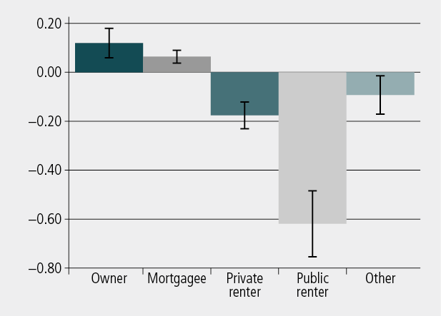
Overall, there was a considerable amount of variation in the receptive vocabulary of children across tenure types. The difference in verbal ability between the children of homeowners and those of public housing tenants was large and statistically significant - about three-quarters of a standard deviation. There were also large differences in verbal ability between children living in public housing and private rental properties. Compared to homeowners and private renters, children in families who double up (the majority of those in "Other" tenure) had levels of verbal ability that were 9% of a standard deviation lower than the mean, significantly higher than those in public housing and 50% greater than those in private rental. The difference between private rental and those in the other tenure was not statistically significant.
Table 6 presents the mean differences in receptive vocabulary for children in the various types of housing tenure, using children of homeowner families as the reference group. These results use regression modelling to take account of child gender, Indigenous status and age, as well as the highest level of parents' education, family structure, mothers' country of birth and equivalised household income.12 To see whether the effect of tenure is sensitive to the age of the child, we present the results separately for children aged 4-5 and 8-9 years.
| Housing tenure type | 4-5 years | 8-9 years |
|---|---|---|
| Owners without a mortgage (reference) | ||
| Owner with a mortgage | -0.02 (0.05) | -0.07 (0.04) |
| Renter - Private landlord | -0.19 ** (0.06) | -0.16 ** (0.06) |
| Renter - State/territory housing authority | -0.67 ** (0.11) | -0.30 ** (0.10) |
| Other landlord/other tenure type | -0.12 (0.07) | -0.08 (0.07) |
| No. of observations | 4,266 | 4,273 |
Notes: OLS regressions take account of child gender, Indigenous status and age, as well as the highest level of parents' education, equivalised household income, family structure and mothers' country of birth. Receptive vocabulary scores are standardised within each age group so that results are comparable across ages. OLS = ordinary least squares. ** p < .01.
In broad terms, the results are very similar to those presented in Figure 1, suggesting that the demographic variables included in the regression modelling are not confounding the simple descriptive results. The level of receptive vocabulary was significantly lower for private renters when compared to homeowners. There was no statistically significant difference between homeowners and those in the "Other" category. Children living in public housing had significantly lower levels of receptive vocabulary compared to children of the same age in families who owned their home outright, albeit to a lesser extent for children aged 8-9 years.
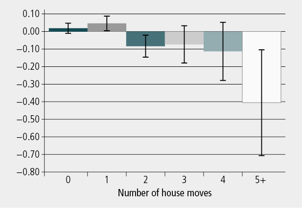
Figure 2 presents mean standardised PPVT scores at Wave 3 according to the number of times the child moved house between 2004 and 2008. The only significant differences in receptive vocabulary were evident when comparing children who had moved once and those who had moved 5 or more times. Those that had moved only once are observed to have levels of receptive vocabulary 5% of a standard deviation higher than the mean (albeit on the cusp of statistical significance) and those who had experienced 5 or more moves have scores 41% of a standard deviation lower than the average.
Figure 2: Receptive vocabulary of children aged 4-5 and 8-9 years, by number of house moves between Wave 1 and Wave 3
Regression modelling of the number of moves for 4-5 and 8-9 year old children, taking into account child and parental demographic variables, indicates a statistically significant effect of 5 or more house moves for children aged 4-5 (see Table 7). This estimate is quite large, suggesting that frequent moves are associated with levels of receptive vocabulary that are 37% of a standard deviation lower than children who reside in the same home for a period of 4 years.
| House moves | 4-5 years | 8-9 years |
|---|---|---|
| None | ||
| One | 0.01 (0.03) | 0.09 * (0.04) |
| Two | -0.04 (0.05) | -0.11 * (0.05) |
| Three | -0.11 (0.07) | 0.05 (0.08) |
| Four | -0.06 (0.10) | 0.12 (0.16) |
| Five or more | -0.37 * (0.18) | -0.16 (0.21) |
| No. of observations | 4,266 | 4,273 |
Notes: OLS regressions take account of child gender, Indigenous status and age, as well as the highest level of parents' education, equivalised household income, family structure and mothers' country of birth. Receptive vocabulary scores are standardised within each age group so that results are comparable across ages. OLS = ordinary least squares. * p < .05.
The estimates for children aged 8-9 appear somewhat less intuitive. A single move is associated with an increase in receptive vocabulary of 9% of a standard deviation compared to stable residency over the previous four years, while an additional move suggests levels of receptive vocabulary that are 11% of a standard deviation lower. One explanation for this might be the lower mobility of those in public housing observed in Table 4. Given the large and statistically significant lower scores observed for these children in Table 6, and keeping in mind that "no moves" is the base case against which we compare the other categories in forming these estimates, it may be the high concentration of children in public housing that are pushing the regression estimates in Table 6 upward.
The lower levels of mobility associated with public housing tenure are, however, unlikely to explain the statistical significance of the negative regression estimates observed for two moves for children aged 8-9, nor the counterintuitive sign on the coefficients for three and four moves. On the other hand, it is possible that these estimates point to a broader need to model tenure choice and residential mobility simultaneously, as in Donkers, Melenberg, van Soest, and Tu (2003). While it may be that housing tenure and residential mobility have an independent effect upon the developmental outcomes of children, tenure choice will in part be the outcome of a family's need, or preference, for mobility. This makes it difficult to interpret the association between tenure, residential mobility and child outcomes, even when all of these appear in the same regression model. Future research could bring more sophisticated statistical techniques, such as those used in Donkers et al. (2003), to bear on this methodological issue.
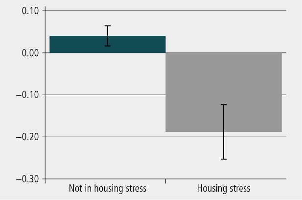
Figure 3 presents mean standardised PPVT scores by housing stress experienced by the children's families. There is a statistically significant difference of just under a quarter of a standard deviation in the level of receptive vocabulary for those who were in housing stress compared to those who were not.
Findings from the regression modelling of the receptive vocabulary of children aged 4-5 and 8-9 years (not shown) suggest that once other demographic characteristics are taken into account, there are no statistically significant differences in the receptive vocabulary of children experiencing housing stress. The results suggest that much of the association between this measure of housing stress and receptive vocabulary reflects having a household income in the bottom 40th percentile rather than having household income in the bottom 40th percentile and high housing costs.
Figure 3: Receptive vocabulary of children aged 4-5 and 8-9 years, by housing stress at Wave 3
Housing and emotional and behavioural problems
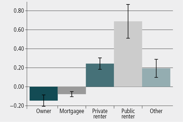
Figure 4 presents the average standardised total SDQ score, a measure of emotional and behavioural problems, by housing tenure type. Children in families who owned their own home had the lowest emotional and behavioural problems, at 15% of a standard deviation below the sample average. Children whose parents were paying off a mortgage also had lower emotional and behavioural problems, at 8% below the mean. Children in families who were living in public housing had the highest emotional and behavioural problems, almost 70% of standard deviation above the mean, which was significantly higher than any other group of children. Children in families who were living in "Other" types of housing had lower levels of emotional and behavioural problems, closer to those observed for children whose families were in private rental (19% and 24% of a standard deviation respectively).
Figure 4: Level of emotional and behavioural problems (SDQ) of children aged 4-5 and 8-9 years, by housing tenure type at Wave 3
presents regression estimates for the standardised total SDQ score for children aged 4-5 and 8-9 years. As in Table 6 children who lived in families who own their own home with no mortgage are the reference case against which comparisons are made. The regressions show that children in families living in public housing had the highest levels of emotional and behavioural problems, even after controlling for family characteristics, at 49% and 63% of a standard deviation higher than children whose parents owned their own home. Children in families who were renting privately also had higher levels of emotional and behavioural problems (23% of a standard deviation for children aged 4-5 and 27% of a standard deviation for children aged 8-9). Those in "Other" tenure had higher emotional and behavioural problems than the average, but somewhat lower than children in private rental, at 17% of a standard deviation for children aged 4-5 years and a quarter of a standard deviation for children aged 8-9 years. Only children aged 8-9 in families whose parents were paying off a mortgage were found to have levels of emotional and behavioural problems that were significantly different from those whose families owned their home outright.
| Housing tenure type | 4-5 years | 8-9 years |
|---|---|---|
| Owners without a mortgage (reference) | ||
| Owner with a mortgage | -0.02 (0.05) | 0.12 ** (0.04) |
| Renter - Private landlord | 0.23 ** (0.07) | 0.27 ** (0.06) |
| Renter - State/territory housing authority | 0.49 ** (0.14) | 0.63 ** (0.13) |
| Other landlord/other tenure type | 0.17 * (0.08) | 0.25 ** (0.08) |
| No. of observations | 3,821 | 3,798 |
Notes: OLS regressions take account of child gender, Indigenous status and age, as well as the highest level of parents' education, equivalised household income, family structure and mothers' country of birth. Receptive vocabulary scores are standardised within each age group so that results are comparable across ages. OLS = ordinary least squares. * p < .05; ** p < .01.
Figure 5 presents the average standardised SDQ scores by the number of house moves experienced between 2004 and 2008. The figure suggests statistically significant increases in emotional and behavioural problems with the number of house moves up to four moves. While not a statistically significant difference, children who had experienced five or more moves had a higher level of emotional and behaviour problems compared to the overall average. Children who were yet to experience a house move at Wave 3 were observed to have total SDQ scores that were 6% of a standard deviation lower than the mean, while children who had experienced four moves were found to have level of emotional and behavioural problems that were just over a quarter of a standard deviation higher than the average. Given the small number of children experiencing five or more moves observed in Table 2, it is not surprising that the estimates at five or more moves are not statistically significant at the 5% level.
Figure 5: Level of emotional and behavioural problems (SDQ) of children aged 4-5 and 8-9 years, by number of house moves between Wave 1 and Wave 3
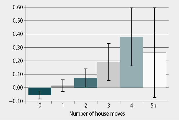
The results from the regression support an increasing relationship between emotional and behavioural problems and number of house moves, but only for children aged 4-5 (Table 9). For older children, it would appear that the variation in total SDQ scores more likely reflects the characteristics of highly mobile families rather than residential mobility per se.
| House moves | 4-5 years | 8-9 years |
|---|---|---|
| None | ||
| One | 0.08 * (0.04) | -0.01 (0.04) |
| Two | 0.08 (0.05) | 0.06 (0.06) |
| Three | 0.27 ** (0.1) | -0.01 (0.1) |
| Four | 0.28 * (0.13) | 0.21 (0.17) |
| Five or more | 0.22 (0.18) | 0.07 (0.29) |
| No. of observations | 3,821 | 3,798 |
Notes: OLS regressions take account of child gender, Indigenous status, age as well as the highest level of parents' education, equivalised household income, family structure and mothers' country of birth. Receptive vocabulary scores are standardised within each age group so that results are comparable across ages. OLS = ordinary least squares. * p < .05; ** p < .01.
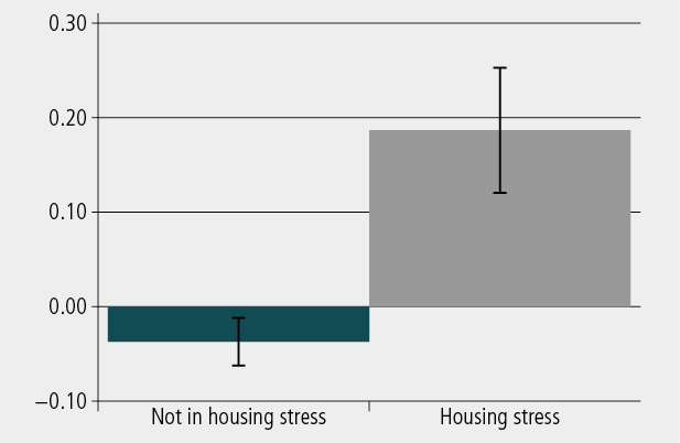
Figure 6 shows the average level of emotional and behavioural problems by housing stress experienced by children's families at Wave 3. The figure indicates that children living in housing stress have levels of emotional and behavioural problems that are a quarter of a standard deviation higher than those not in housing stress.
The regression models examining the association between housing stress and children's emotional and behavioural problems (not shown but available from the authors upon request) are consistent with the results for receptive vocabulary. Once low household income is taken into account, housing stress is not associated with statistically significant variation in emotional and behavioural problems.
Figure 6: Level of emotional and behavioural problems of children aged 4-5 and 8-9 years, by housing stress at Wave 3
Discussion and conclusion
Findings from this study begin to fill the gap in our understanding of the influence of housing on children's development and the housing circumstances of young Australian families.
The third wave of LSAC, when study children were aged 4-5 and 8-9 years, represents a sample of families that are relatively young. It is therefore not surprising that the majority (61%) of these families were observed to be partway through paying off a mortgage. At this time:
- a non-trivial proportion of families did, in fact, own their homes outright (13%);
- private rental was the second most common tenure type at Wave 3 (16%);
- the remaining LSAC families were in public housing (3.2%) or doubling up; that is, "Other" tenure (7%).
The majority of children did not move house between 2004 and 2008 (55%), and most children who experienced a house move did so only once (27%); however, a significant minority experienced two or more moves (18%).
While families who own their home outright do not incur any out-of-pocket expenses associated with their tenure aside from rates and maintenance:
- "Other" tenure had an average cost of $107 a week;
- renting from a state/territory housing authority cost $160 per week;
- private rentals cost just under $300 per week; and
- families with mortgages faced costs of $434 a week, the highest of all groups.
There were some very large differences in children's developmental outcomes by type of housing tenure and house moves, but not for housing stress after controlling for the low-income status of these households. The evidence from the regression modelling in particular suggests that the largest differences in levels of receptive vocabulary and emotional and behavioural problems are found when examining the housing tenure type of childrens' families. Children in families who were living in public housing had lower levels of receptive vocabulary and higher levels of emotional and behavioural problems than children living in families who owned or were paying off their own home. Interestingly, it appears that the cognitive outcomes of children aged 4-5 are more sensitive to tenure than emotional and behavioural problems, while the opposite seems true for children aged 8-9.
Residential mobility does not appear to be strongly associated with the receptive vocabulary or the emotional and behavioural problems of children aged 8-9. While the level of residential mobility of children in the LSAC sample was not very high, many studies have found statistically significant differences using a lifetime number of moves of three or more for adolescents (Jelleyman & Spencer, 2008). Perhaps the distance moved and whether children shifted schools may be one explanation for the lack of differences in the Australian context. We do, however, find statistically significant differences in both receptive vocabulary and emotional and behavioural problems for children aged 4-5. This might suggest that this is a more sensitive period in a child's development, where continuity of the community and school environment may be more important than at later stages in a child's life. Future research could examine this conjecture.
While this is one of few Australian studies to use nationally representative data to study the influence of housing on children's development it is not without its limitations.13 It is important to note that the associations between children's development and housing tenure cannot be considered to be causal. This paper has shown that there are very large differences in the housing costs of different tenure types, and therefore differences in the types of families who choose different types of tenure. While the regression models have taken account of many of these variables (child gender, age and Indigenous status; highest level of parental education; household income; mother born overseas), there may be others that explain these significant associations. To identify causal effects of housing on children's development, examining differences in the availability of types of housing across Australian states and territories may offer the best approach.
Having a "home" is a fundamental need of all children. Findings from this research suggest that the developmental outcomes of children may be more sensitive to residential mobility between the ages of 4 and 5, and that living in types of housing tenure associated with instability (such as doubling up) is associated with some adverse effects. Even more substantive is the role played by the type of housing tenure, with those children living in public housing having much worse receptive vocabulary and much higher levels of emotional and behavioural problems than children in other types of housing. One explanation is that to be eligible for public housing, families need to have significant and ongoing needs, whereas a doubling-up arrangement can be entered into fairly quickly at a time of temporary housing insecurity. Housing costs may be another possible explanation, as families who are doubling-up with relatives and those living in public housing have much lower housing costs. Compared to those living in public housing, those who were doubling up had housing costs that were $55 per week lower. Given that there were more limited adverse outcomes for these children compared to those in public housing, it is perhaps possible that the smaller financial burden of this form of tenure is a reason for this finding.
Further work could examine the role of the financial stress associated with renting and having a mortgage, which dilutes the financial resources that low-income parents have to provide resources for their children. Learning more about the influence of financial stress on the mental health and parenting behaviours of low-income parents would help to ensure that housing policy works to enhance the wellbeing and development of Australian children.
Endnotes
1 The Journeys Home study at the Melbourne Institute of Applied of Economics and Social Research (in its second wave at the time or writing) represents an exciting new resource for examining the residential mobility of families experiencing housing instability. However, the publications produced from this study do not yet quantify the extent of this mobility. For further information on Journeys Home, see <www.melbourneinstitute.com/journeys_home/>.
2 The latter percentage is based on the authors' calculations, using Table 2 of Australian Bureau of Statistics (ABS, 2009).
3 We focus on the non-attriting sample because the Wave 3 questionnaire asked parents who had not responded to Wave 2: "How many homes has the child lived in the last two years?". We cannot therefore ascertain the housing mobility these children may have experienced over the two years following the first data collection.
4 This question was not asked in Wave 1.
5 Equivalised household income is an estimate of financial living standards in which the incomes of different households are adjusted according to an estimate of their costs, taking into account economies of scale. The results presented in this figure are based on the so-called "modified OECD scale", which gives a weight of 1.0 to the first adult in the household, a weight of 0.5 for each additional adult (people aged 15 years and over) and a weight of 0.3 for each child. (For example, it is assumed that a single parent with two children under 15 years old requires 1.6 times the disposable income of a person living alone in order to have the same living standard.) The total household income is then divided by the household weight to produce equivalised household income.
6 We use the SIH household weights in estimating the bottom 40th percentile cut-off.
7 It is also worth noting that the money that could be earned by homeowners were they to rent out their home in the private rental market and acquire housing services elsewhere does, of course, constitute an opportunity cost. However, it is out-of-pocket housing costs that are the focus of this study.
8 We control for household income using a binary indicator of whether the household is in the bottom two quintiles of household income for the wave.
9 The specific version of the PPVT used in LSAC uses a book of 40 display pictures. The child points to (or says the number of) a picture that best represents the meaning of the word read out by the interviewer.
10 There is also an additional SDQ subscale that measures prosocial behaviour. We excluded this since it is not one of the subscales used in the formation of the total SDQ scale.
11 In more technical terms were repeated samples to be taken from the population of interest we would expect that 95% of the averages calculated from these samples would lie within these bounds.
12 We operationalised the equivalised household income measure via a dummy variable indicating whether families were in the bottom 40% of the equivalised household income distribution. Given that labour force status is very closely associated with household income, we included parents' labour force status.
13 A recent publication by Maguire, Edwards, and Soloff (2012) examined transitions in tenure and overcrowding across the first 3 waves of LSAC.
References
- Aaronson, D. (2000). A note on the benefits of homeownership. Journal of Urban Economics, 47, 356-69.
- Astone, N. M., & McLanahan, S. S. (1994). Family structure, residential mobility, and school dropout: A research note. Demography, 31, 575-583.
- Australian Bureau of Statistics. (2007). Survey of Income & Housing 2007-08: Paper questionnaire. Canberra: ABS.
- Australian Bureau of Statistics. (2009). Housing occupancy and cost 2007-08 (Cat. No. 4130.0). Canberra: ABS.
- Australian Institute of Health and Welfare. (1999). SAAP national data collection accompanying children report 1998 Australia (AIHW Cat. No. HOU 39). Canberra: AIHW.
- Australian Housing and Urban Research Institute. (2006). How does security of tenure impact on public housing tenants? (Research and Policy Bulletin No. 78). Melbourne: AHURI. Retrieved from <www.ahuri.edu.au/publications/download/rap_issue_78>.
- Bartfield, J., & Dunifon, R. (2005). State-level predictors of food insecurity and hunger among households with children (Contractor and Cooperator Report No 13). Retrieved from <hdl.handle.net/10113/32791>.
- Bartholomew, T. (1999). A long way from home: Family homelessness in the current welfare context. Geelong: Deakin University Press.
- Boehm, T. P., & Schlottman, A. M. (1999). Does home ownership by parents have an economic impact on their children? Journal of Housing Economics, 8(3), 217-232.
- Boyle, M. H. (2002). Home ownership and the emotional and behavioral problems of children and youth. Child Development, 73(3), 883-892.
- Chamberlain, C., Johnson, G., & Theobald, J. (2007). Homelessness in Melbourne. Melbourne: RMIT Publishing.
- Chamberlain, C., & MacKenzie, D. (1998). Youth homelessness: Early intervention and prevention. Sydney: Australian Centre for Equity Through Education.
- Chamberlain, C., & Mackenzie, D. (2008). Counting the homeless 2006. Canberra: Australian Bureau of Statistics.
- Conger, R. D., & Donnellan, M. B. (2007). An interactionist perspective on the socioeconomic context of human development. Annual Review of Psychology, 58, 175-199.
- Dockery, A. M., Kendall, G., Li, J. H., Mahendran, A., Ong, R., & Strazdins, L. (2010). Housing and children's development and wellbeing: A scoping study (AHURI Final Report No. 149). Melbourne: Australian Housing and Urban Research Institute.
- Donkers, B., Melenberg, B., van Soest, A. & Tu, Q. (2003) Modelling mobility and housing tenure choice: A multinomial probit model for panel data. Unpublished manuscript, Tilburg University, Netherlands.
- Edwards, B. (2005). Does it take a village? An investigation of neighbourhood effects on Australian children's development. Family Matters, 72, 36-43.
- Edwards, B., & Bromfield, L. M., (2009). Neighborhood influences on young children's conduct problems and pro-social behavior: Evidence from an Australian national sample. Children and Youth Services Review, 31, 317-324.
- Edwards, B., & Maguire, B. (2012). Parental mental health. In B. Maguire, & B. Edwards (Eds.), The Longitudinal Study of Australian Children annual statistical report 2011 (pp. 7-17). Melbourne: Australian Institute of Family Studies. Retrieved from <www.growingupinaustralia.gov.au/pubs/asr/2011/asr2011b.html>.
- Evans, G. W. (2006). Child development and the physical environment. Annual Review of Psychology, 57, 423-451.
- Fogelman, K., Fox, A., & Power, C. (1989). Class and tenure mobility: Do they explain social inequalities in health among young adults in Britain? In J. Fox (Ed.), Health inequalities in European countries (pp. 333-352). Aldershot, UK: Gower.
- Goodman, R. (1997). The Strengths and Difficulties Questionnaire: A research note. Journal of Child Psychology and Psychiatry, 38, 581-586.
- Green, R., & White, M. (1997). Measuring the benefits of home owning: Effects on children. Journal of Urban Economics, 41, 441-461.
- Harkness, J., & Newman, S. J. (2005). Housing affordability and children's well-being: Evidence from the National Survey of America's Families. Housing Policy Debate, 16(2), 635-666.
- Harkness, J., Newman, S., & Holupka, S. (2009). Geographic differences in housing prices and the well-being of children and parents. Journal of Urban Affairs, 31(2), 123-146.
- Haurin, D. R., Parcel, T. L., & Haurin, R. J. (2002). Does homeownership affect child outcomes? Real Estate Economics, 30(4), 635-666.
- Jelleyman, T., & Spencer, N. (2008). Residential mobility in childhood and health outcomes: A systematic review. Journal of Epidemiology and Community Health, 62, 584-592.
- Johnson, G., Gronda, H., & Coutts, S., (2008). On the outside: Pathways in and out of homelessness. Melbourne: Australian Scholarly Publishing.
- Kane, P., & Garber, J. (2004). The relations among depression in fathers, children's psychopathology, and father-child conflict: A meta-analysis. Clinical Psychology Review, 24, 339-360.
- Lovejoy, M. C., Grazcyk, P. A., O'Hare, E., & Neuman, G. (2000). Maternal depression and parenting behaviour. Clinical Psychology Review, 20, 561-592.
- Maguire, B., Edwards, B., & Soloff, C. (2012). Housing characteristics and changes across waves. In Australian Institute of Family Studies, Longitudinal Study of Australian Children Annual statistical report 2011 (pp. 67-77). Melbourne: AIFS.
- McCaughey, J. (1992). Where now? Homeless families in the 1990s (Policy Background Paper No. 8). Melbourne: Australian Institute of Family Studies.
- Park, J. M., Fertig, A., & Allison, P. (2011). Physical and mental health, cognitive development, and health care use by housing status of low-income young children in 20 American cities: A prospective cohort study. American Journal of Public Health. doi:10.2105/AJPH.2010.300098
- Phillips, B. (2011). The great Australian dream: Just a dream (AMP:NATSEM Report No. 29). Canberra: National Centre for Social and Economic Modelling. Retrieved from <www.natsem.canberra.edu.au/publications/?publication=the-great-australian-dream-just-a-dream>.
- Sharfstein, J., & Sandel, M. (1998). Not safe at home: How American's housing crisis threatens the health of its children. Boston: Boston Medical Centre, Department of Pediatrics.
- Simpson, G. A., & Fowler, M. G. (1994). Geographic mobility and children's emotional/behavioral adjustment and school functioning. Pediatrics, 93(2), 303-309.
- Wilson, S., & Durbin, C. E. (2010). Effects of paternal depression on fathers' parenting behaviors: A meta-analytic review. Clinical Psychology Review, 30, 167-180.
- Wood, D., Halfon, N., Scarlata, D., Newacheck, P., & Nessim, S. (1993). Impact of family relocation on children's growth, development, school function, and behavior. Journal of the American Medical Association, 270(11), 1334-1338.
- Yates, J. (2007). Housing affordability and financial stress (AHURI Research Paper No. 6). Melbourne: Australian Housing and Urban Research Institute.
- Yates, J. & Gabrielle, M. (2006). Housing affordability in Australia (National Research Venture 3: Housing Affordability for Lower Income Australians Research Paper No. 3). Sydney: Australian Housing and Urban Research Institute.
Taylor, M., & Edwards, B. (2012). Housing and children's wellbeing and development: Evidence from a national longitudinal study. Family Matters, 91, 47-61.
19 December 2012