The tyrannies of distance and disadvantage
Factors related to children's development in regional and disadvantaged areas of Australia
You are in an archived section of the AIFS website
Overview
This research report investigates whether children in regional areas experience a "tyranny of distance" or a "tyranny of disadvantage".
In other words, are the gaps in children's development in regional areas compared to children living in the major cities explained by their distance from the major cities (remoteness), or is it because many regional areas are disadvantaged compared to the cities?
The analyses make use of data from Growing up in Australia: The Longitudinal Study of Australian Children (LSAC) to report on differences in family demographic and economic characteristics, parent wellbeing and parenting style, family social capital and access to services, and children's educational activities, and to relate those differences to how children are developing. The study includes children aged from 0-1 up to 8-9 years old.
Key messages
-
There is a tyranny of distance or disadvantage but it depends on the outcome examined.
-
There were enduring differences in child cognitive outcomes by whether children live in major city areas compared to regional areas, even after a broad range of other factors are taken into account, indicating that there is a tyranny of distance for cognitive outcomes.
-
There was also a tyranny of disadvantage for child emotional or behavioural problems. The findings suggest that children living in disadvantaged areas experience greater emotional or behavioural problems, even when all other factors are taken into account.
-
Findings from the current study provide the first systematic national information on a broad range of child outcomes, as well as a large number of other variables that are known to shape children's development, which could vary depending on geographic locality or level of disadvantage.
Executive summary
Families living in regional or rural areas of Australia can face challenges that may be less commonly experienced by families in major cities; for example, in accessing services and good-quality infrastructure. It is important to understand whether these different experiences and other differences in family life associated with living in regional areas have implications for children's development. Further, within geographically defined localities of Australia, some are more socio-economically disadvantaged than others. The level of socio-economic disadvantage in the local area in which children live is known to influence children's development, though it is not understood whether children living in disadvantaged major city areas have different experiences and outcomes compared to children living in disadvantaged regional areas.a
This report examines whether what children in regional areas experience is a "tyranny of distance" or a "tyranny of disadvantage". In other words, are the gaps in children's development in regional areas compared to children living in the major cities explained by their distance from the major cities (remoteness), or is it because many regional areas are disadvantaged compared to the cities? The analyses make use of data from the first three waves of Growing Up in Australia: The Longitudinal Study of Australian Children (LSAC) to report on differences in neighbourhood, family, social, educational and other contexts for children, and to relate those differences to how children are developing. The study includes children aged from 0-1 up to 8-9 years old, and therefore provides useful insights into issues of relevance to families with children in their early years.
The current study compares families and children living in different areas of Australia, first defined according to their remoteness (major cities, inner regional areas and outer regional areas), and then according to their level of disadvantage (defined using local area unemployment rates). While an important group, children from remote parts of Australia are not included in the current study, as they are not represented in sufficient numbers in LSAC to obtain robust statistical estimates. Throughout the report, comparisons are thus made across the following socio-geographic areas:
- major city areas with low unemployment rates;
- major city areas with high unemployment rates;
- inner regional areas with low unemployment rates;
- inner regional areas with high unemployment rates;
- outer regional areas with low unemployment rates; and
- outer regional areas with high unemployment rates.
The main question we sought to answer was how children's outcomes vary by geographic locality and by disadvantage. We examined two cognitive outcomes - receptive vocabulary and non-verbal reasoning - and two other outcomes - the risk of experiencing clinically significant emotional or behavioural problems and of being overweight.
Differences in local area characteristics, family demographics, parent wellbeing and parenting, social capital and access to services, and educational activities between geographic localities, or between disadvantaged and advantaged areas might be part of the explanation for any differences in child wellbeing that were observed, so we also provide information here on these characteristics for each of the six socio-geographic areas.
Contexts for child development
We focused on how the following contexts vary according to the remoteness and disadvantage of different areas across Australia:
- family demographic and economic characteristics;
- parent wellbeing and parenting style;
- family social capital and access to services; and
- children's educational activities.
The key findings from each context are discussed in more detail below. Together, there are a number of key differences in contexts that may be relevant to children's development according to geographic locality and level of disadvantage, which may be reflected in how children grow and develop. One of the important features of these factors is that many are amenable to change, and therefore could be the targets of policies and service delivery.
Family demographic and economic characteristics
Advantaged areas in major cities stood apart from the other areas examined when focusing on family demographic and economic characteristics. On many measures, the circumstances of these families differed from those in disadvantaged major city areas, as well as from those in inner and outer regional areas. Differences according to disadvantage were also apparent in inner and outer regional areas, although the advantage/disadvantage disparity was not as great as it was in major city areas. For example, the percentages of single parents, mothers with a university education and mothers born overseas were similar in both disadvantaged and advantaged regional areas, but rates were different in advantaged and disadvantaged areas in the major cities. The percentage of jobless families and those experiencing financial hardship were more similar in disadvantaged and advantaged regional areas than in advantaged and disadvantaged major city areas, where there was a greater discrepancy.
Parent wellbeing and parenting style
In terms of parent wellbeing and parenting style, there were fewer differences. There were no differences by geographic locality or level of disadvantage in terms of mental health and relationship hostility. Fathers had much higher rates of risky binge drinking in regional areas, particularly in outer regional areas, than in major city areas; but though these rates were high, they were consistent with other studies (e.g., Miller, Coomber, Staiger, Zinkiewicz, & Toumbourou, 2010). There were differences by locality and level of disadvantage for mothers and fathers being overweight. For mothers, a higher proportion was overweight in regional areas, as well as in disadvantaged areas (regardless of locality), with the highest percentage being those in disadvantaged outer regional areas. On the other hand, for fathers, the highest levels of being overweight were in inner regional areas. In outer regional areas, higher proportions of fathers were overweight in advantaged compared to disadvantaged areas. There was little difference in parenting styles of mothers and fathers between geographic localities or between disadvantaged and advantaged areas.
Family social capital and access to services
Some measures of social capital and service use for children did not vary according to areas of remoteness and disadvantage, but there were some protective factors for parent and child wellbeing that were higher in regional areas than in major cities, such as involvement in community organisations, sense of neighbourhood belonging and safety, and obtaining help from family and friends. Also, ratings of neighbourhood quality - including parents' perceptions of safety and parents' involvement in volunteer or community groups - were higher in advantaged areas than in disadvantaged areas.
Children's educational activities
Children's educational activities are likely to be shaped by parents' aspirations for their children's learning, and by their employment arrangements, which can mean parents have varying needs for child care. There were some differences in children's educational activities in the home, with fewer children living in disadvantaged areas having 30 or more children's books in the home and being read to daily than in advantaged areas. Children's television viewing was also marked by consistent differences between advantaged and disadvantaged areas for all ages, with children living in disadvantaged areas being more likely to watch a greater amount of television. Within major city areas, differences between disadvantaged and advantaged areas were most apparent; however, high levels of television viewing were similar in both advantaged and disadvantaged areas in inner and outer regional areas. Also, those children in disadvantaged areas of the major cities were less likely to be enrolled in outside-school-hours care, or to participate in other outside-school activities. There were no consistent differences in children's attendance at child care between geographic localities or between disadvantaged and advantaged areas, and rates of preschool attendance were consistently high across all socio-geographic areas.
Child outcomes
The key question of the report is the extent to which children's outcomes are shaped by a tyranny of distance (differences between geographic localities) or by a tyranny of disadvantage (differences between areas with higher compared to lower levels of unemployment). Findings from the current study provide the first systematic national information on a broad range of child outcomes, as well as a large number of other variables that are known to shape children's development, which could vary depending on geographic locality or level of disadvantage.
Is there a tyranny of distance or disadvantage? The answer to this question depends on the outcome examined. The evidence seems to suggest that there are enduring differences in child cognitive outcomes by whether children live in major city areas compared to regional areas, even after a broad range of factors are taken into account, indicating that there is a tyranny of distance for cognitive outcomes.
There was also a tyranny of disadvantage for child emotional or behavioural problems. The findings suggest that children living in disadvantaged areas experience greater emotional or behavioural problems, even when all other factors are taken into account. While there were differences by disadvantage between children's levels of cognitive and physical outcomes when not adjusting for other demographic characteristics, these differences could be partly or wholly explained by the demographic composition of families and aspects of the children's social context, including parenting and social capital.
A note of caution in the interpretation of findings from the statistical modelling is warranted, as the modelling precludes causal explanations, even though there was a rich set of variables included.
Study implications
Turning to the study implications, the authors ask what the role of location-based approaches is in the development of service delivery and policy. First, an important point should be made about having location-based services targeted at families living in disadvantaged areas. Even if there are no additional effects of disadvantaged areas over and above the demographic composition of families living in such areas, these types of policies should be considered, as they offer an effective means of planning and targeting services to disadvantaged families. Clearly, in instances where there are persistent differences between disadvantaged and advantaged areas even after a large number of other factors are taken into account - such as is the case with children's emotional or behavioural problems - then there is an additional reason and benefit to targeting services in areas of high unemployment.
In the case of geographic localities, a focus on enhancing the learning environments of children may be important, given that findings from this study also suggest that there were persistent differences in children's cognitive outcomes between the major cities and regional areas that were not explained by the rich set of variables that were included in the statistical models. Enhancing the early education experiences of children and improving the quality of primary school education, as well as getting parents more involved in children's education at home (such as through reading programs) may be important in addressing the "gap" between children's cognitive outcomes in the major cities and in regional areas.
To understand differences in children's outcomes between geographic localities, it is important to note that academic achievement and cognitive development are not the only predictors of positive development, and that on other factors - such as emotional or behavioural problems and overweight or obese - there were no differences between geographic localities once other factors were taken into account in the statistical models. Moreover, high levels of achievement may be important if children wish to attend university, but in many occupations, tertiary qualifications are not relevant. In other studies of rural areas, adolescents learned independence, leadership and social skills by interacting with their family through working on farms, engaging in extracurricular activities and community groups, and taking up leadership positions in these community groups (Elder & Conger, 2000). Many of these skills are transferable to jobs that may be more prevalent in regional areas.
It is important to be mindful that children's development occurs in different environmental contexts, and the development of policies and delivery of services need to be nuanced to cater to the different needs and strengths of children growing up in this "wide brown land".
Footnote
a For the sake of clarity, the terms "geographic locality" or "locality" are used in this report to refer generically to the three areas defined by remoteness: major city, inner regional and outer regional. "Socio-geographic areas" is used to refer generically to the six areas defined by remoteness ´ disadvantage. "Regional areas" is used when referring to both the inner and outer regional areas (but not the major cities).
1. Introduction
There is growing awareness that issues faced by families living in regional or rural areas of Australia are not necessarily the same as those faced by families living in major cities. Differential access to services and infrastructure, along with different social and demographic characteristics of the various geographic localities of Australia make it essential for us to understand whether such differences have implications for children. Further, there are many areas in Australia that are socio-economically disadvantaged. The level of disadvantage in the local area in which children live is known to influence children's development, although it is not understood whether children living in disadvantaged major city areas have different experiences and outcomes compared to children living in disadvantaged regional or rural areas.1
This report examines whether what children in regional areas experience is a "tyranny of distance" or a "tyranny of disadvantage". In other words, are the gaps in children's development in regional areas compared to children living in the major cities explained by their distance from the major cities (remoteness), or is it because many regional areas are disadvantaged compared to the cities? The analyses make use of data from the first three waves of Growing up in Australia: The Longitudinal Study of Australian Children (LSAC) to report on differences in neighbourhood, family, social, educational and other contexts for children, and to relate those differences to how children are developing. The study includes children aged from 0-1 up to 8-9 years old, and therefore provides useful insights into issues of relevance to families with children in their early years.
The current study compares families and children living in different areas of Australia, first defined according to their remoteness (major cities, inner regional areas and outer regional areas), and then according to their level of disadvantage (defined using local area unemployment rates). The remoteness measure we use is based upon an underlying Accessibility/Remoteness Index of Australia Plus (ARIA+) score, which is derived from information about road distances from major service centres (Glover & Tennant, 2003). While a very important group, children from very remote parts of Australia are not included in the current study, as they are not represented in sufficient numbers in LSAC to obtain robust statistical estimates. Throughout the report, comparisons are made thus across the following socio-geographic areas:
- major city areas with low unemployment rates;
- major city areas with high unemployment rates;
- inner regional areas with low unemployment rates;
- inner regional areas with high unemployment rates;
- outer regional areas with low unemployment rates; and
- outer regional areas with high unemployment rates.
Comparisons between regional areas and major cities often ignore levels of socio-economic disadvantage, which can be significant in regional areas. The focus of this report is to highlight issues faced by children in regional areas and children in disadvantaged areas, and therefore the literature that follows (Section 2) concentrates on what is known on these topics.
The structure of the report is as follows. Section 2 provides a brief review of the literature on the geographic distribution and demography of the Australian population, socio-economic changes in regional areas in Australia, geographic location and child development, and local area disadvantage and child development. Section 3 describes the data and methods used in the study. Sections 4 to 8 analyse the characteristics of families and children who live in the six socio-geographic areas described above that might potentially explain differences in child outcomes. Section 4 focuses on differences in the local area, such as the socio-demographic characteristics of the area and parents' ratings of neighbourhood quality. Section 5 reports on family demographic and economic characteristics, including family form, maternal education, employment status of parents, country of birth, financial hardship and housing tenure. In Section 6, differences in parent wellbeing and parenting are documented. Social capital - the social connections between people in the neighbourhood that encourage trust, support and understanding (Stone, 2001) - and the services that are available to families in each of the six socio-geographic areas is examined in Section 7. Section 8 provides information on children's education, both in the home (books, reading by parents, TV watching and educational expectations) and outside the home (child care and preschool). Section 9 focuses on the key research question of whether a tyranny of distance or disadvantage affects children's outcomes. It describes differences in learning, social and emotional wellbeing and physical health between children living in the six socio-geographic areas, while taking into account many of the characteristics described in Sections 4 to 8. Section 10 discusses the overall findings and implications of the study.
Footnote
1 For the sake of clarity, the terms "geographic locality" or "locality" are used in this report to refer generically to the three areas defined by remoteness: major city, inner regional and outer regional. "Socio-geographic areas" is used to refer generically to the six areas defined by remoteness × disadvantage. "Regional areas" is used when referring to both the inner and outer regional areas (but not the major cities).
2. Literature review
2.1 Geographic distribution and demography of the Australian population
According to 2011 Australian Census data, seven in ten (70%) Australians live in major cities, almost one in five (18%) live in inner regional areas, almost one in ten (9%) in outer regional areas and around one in forty live in remote or very remote areas (1.6% remote and 1.1 % very remote).2
Largely as a result of the decline in the agricultural sector, the proportion of the Australian population living outside the capital cities declined from the early 1900s to the 1970s'in 1906, 63% of the population lived outside of the capital cities, and this fell to about 36% by 1976 (Australian Bureau of Statistics [ABS], 2007). Since then, the regional population has been relatively stable. From 1996 to 2006, there was a small increase in population growth in inner regional areas (0.8%), but the number of people living in outer regional areas was stable (ABS, 2008). There was similarly little change between 2006 and 2011 in the distribution of the population across regional areas, with the percentages in 2006 in each of the remoteness areas being very similar to those given above for 2011 (see Baxter, Gray & Hayes, 2011).
There have been considerable changes in population distribution within Australia. One particularly noteworthy change is the movement of the population towards coastal areas, referred to as a 'sea change'. Major provincial centres and towns around capital cities have also experienced growth, largely reflecting the relocation of retirees, lifestyle changes, high city house prices and an increased prevalence of jobs where people can work remotely from home (ABS, 2007). Another very significant factor in the growth of regional towns has been the flourishing mining industry, which has led to significant increases in the population of those areas involved in that business.
2.2 Socio-economic changes in regional areas in Australia
Although not the focus of this study, it is important to review recent socio-economic changes that have occurred in regional areas in Australia. The decline in the importance of agriculture over the last few decades has been a key one of these. The reduction in the terms of trade for primary produce such as wheat, wool and barley that began in the mid-1970s has continued through the 2000s (Productivity Commission, 2009), and the droughts in 2002-03 and 2006-10 accelerated the associated decrease in agricultural employment in inner and outer regional and remote areas (Edwards, Gray & Hunter, 2009; Productivity Commission, 2009). Analysis of the 2001 and 2006 Census of Population and Housing by the Productivity Commission (2009) showed that over that period the share of people employed in agriculture reduced by 2% in inner regional areas and 3% in outer regional and remote areas. This was particularly important for outer regional and remote areas, as in those areas agriculture employed more people than mining and manufacturing combined.
While the number of farms has decreased, the average farm size has increased. There were 196,000 farms in 1968-69, but by 2004-05 this had dropped to 130,000. Over the same period, the average farm size increased from around 2,500 hectares to 3,400 hectares, and the concentration of agricultural output from the largest farms also increased (Productivity Commission, 2009).
Further analysis of the Census of Population and Housing has provided a more nuanced perspective on those regional areas that have been economic winners and losers (Baum, Haynes, Gellecum, & Han, 2007). Based on the 2001 Census, advantaged areas include the mining regions, areas with high levels of amenity or tourism, and those that have important regional and rural service functions. In terms of disadvantage, Baum et al. described regional areas that were characterised by poor labour market outcomes, high levels of financial stress, and household joblessness; these were usually in areas where there had been high levels of manufacturing supported by protectionism. Also described as being disadvantaged were areas with high levels of employment in agriculture but with far more low-income than high-income earners, and the 'income poor but asset rich' amenity-based areas on the coasts of NSW and Queensland that are characterised by high levels of internal migration by retirees and welfare recipients.
Tony Vinson's (2007) Dropping Off the Edge report documented areas of concentrated disadvantage across Australia, based on the indicators of low income, high rates of disability, elevated levels of criminal convictions, poorer economic conditions (unskilled workers, long-term unemployment, limited computer use/access to Internet), and low educational attainment (incomplete secondary education, early school leaving). Vinson identified areas of disadvantage in Victoria, New South Wales, Queensland, South Australia, Western Australia and the Northern Territory, and found that across the five largest states, 52% of the 170 disadvantaged locations were in rural areas (60% in Queensland, 48% in New South Wales, 33% in Victoria, 60% in South Australia and 70% in Western Australia). This highlights that in Australia, locational disadvantage is as much an issue for regional and rural areas as it is for the major cities.
2.3 Geographic location and child development
There has been limited research comparing children's development in regional and rural areas of Australia with that of those living in cities, with a particular gap existing in data available from large-scale national studies. Bell and Merrick (2009), in an editorial about rural child health, stated: 'There is an urgent need to develop an existing body of research on the needs of rural and remote children and adolescents' (p. 86).
Recent analyses using LSAC data for 8-9 year old children, showed that some differences are apparent in outcomes for children in regional areas (Baxter, Gray, & Hayes, 2011). In terms of learning or cognitive outcomes, children were doing best in major cities, followed by inner regional areas and then outer regional areas. For physical outcomes, children in inner regional areas were somewhat less likely to have very good outcomes compared with children in outer regional areas or major cities. Socio-emotional outcomes were not found to vary across geographic localities; however, these analyses were intended to provide a broad overview of these data and did not examine the reasons for such differences.
The Australian Institute of Health and Welfare (AIHW; 2009) report, A Picture of Australia's Children, brought together some national information on differences in outcomes of children by geographic locality. For example, data on child mortality for the period 2004-06 suggest there were some differences by locality'rates of death for infants (under 1 year) in major cities (about 4 per 1,000 live births) were significantly lower than in inner regional and outer regional areas (about 5 and 6 per 1,000 live births respectively). The rates of death per 100,000 for children aged 1-14 years were also higher in inner and outer regional areas compared to major cities (although the difference was only statistically significant for outer regional areas).
The National Assessment Program'Literacy and Numeracy (NAPLAN) provides national data on the academic achievement of Australian students by locality. In 2010, there were consistent differences between Year 3 students by geographic location, with children living in metropolitan areas having better mean scores on reading, writing, language conventions and numeracy when compared to children living in provincial and remote areas (Australian Curriculum Assessment and Reporting Authority [ACARA], 2010). This was the case even when the sample was restricted to children who were not Indigenous.
Analysis of the 2007 Australian National Children's Nutrition and Physical Activity Survey suggests that the prevalence of overweight and obesity in children aged 2-12 years is higher among children living in inner regional areas (24%) than in major cities (22%) and outer regional and remote areas (22%) (AIHW, 2009). However, a smaller study of 636 children aged 5-12 years residing in rural and urban areas of Victoria found no significant differences in the percentage of children who were overweight or obese (29% in urban areas and 27% in rural areas; Cleland et al., 2010). A New Zealand study of 3,275 children aged 5-15 years, collected as part of the 2002 National Children's Nutrition Survey, reported that urban boys and girls were more likely to be overweight or obese than their rural counterparts (1.3 times for boys and 1.4 for girls; Hodgkin, Hamlin, Ross, & Peters, 2010).
The 2005 ABS Childcare Survey provides some information on rates of attendance at preschool or long day care according to geographic locality. Attendance at preschool or long day care was similar across localities for 4-year-olds; however, 3-year-olds attended at the highest rates in major cities, followed by inner regional areas, and then outer regional and remote areas (AIHW, 2009).
The most notable international longitudinal study of rural children has been the Iowa Youth and Families Project (IYFP; Elder & Conger, 2000). This study followed the lives of 451 children (since seventh grade) and their families from an agricultural area of rural Iowa, United States, from 1989 to 2000. While more focused on adolescence, the IYFP was an important study because it tracked a relatively large sample of families during a period of significant economic change in the agricultural sector. Researchers from the study also developed the family stress model of economic hardship'a theoretical model of how families cope with economic strains and the pathways of influence on children's developmental outcomes. We will use this theoretical model to inform this study and also describe it in this section.
Elder and Conger (2000) reported that, at the time of the study, a significant restructuring of the agricultural sector in Iowa had taken place, similar in nature but greater in scope than what had occurred in Australia over a similar period. Between 1950 and 1990, the number of farms in the study area halved, while the size of the farms doubled. The population declined by 12% over this forty-year period, with the majority of the population loss flowing out of the farm sector. The value of farmland decreased from a high of over US$4,500 per acre in 1978 to US$1,500 per acre in 1987. Other economic indicators also reflected this decline; for example, building permits had reduced to a fraction of the number approved from the 1970s, while retail sales in the area also decreased.
The key findings from the Iowa Youth and Families Project emphasised that how parents coped with economic hardship individually (e.g., mental health) and as a couple (e.g., parental relationships) influenced their ability to parent effectively, and made a difference as to how economic hardships were experienced by their children (Elder & Conger, 2000). The family stress model of economic hardship postulates a series of mediated relationships between financial hardship, parents' mental health, conflict between caregivers, parenting practices and children's mental health (Conger & Donnellan, 2007). In brief, the model proposes that the experience of low income and lack of parental employment influences the number of financial hardship events experienced by the family (e.g., difficulty paying bills, making financial cutbacks, or selling goods to generate income). The experience of financial hardship, in turn, produces elevated levels of parental mental health problems. The negative affect or emotional distress from the adverse experience of financial hardship also produces aggression, in the form of increased conflict in the parental relationship. Both mental health problems and parental relationship conflict are proposed to decrease warm parenting, and increase angry, critical and inconsistent parenting behaviours directed towards children. Although originally developed and tested using data from the IYFP (Conger & Elder, 1994), empirical support for the family stress model of economic hardship has been found in several other studies, using samples representing a broad range of national and ethnic groups, geographic locations and children's ages (for a review of these, see Conger & Donnellan, 2007).
In addition to the role of the family factors discussed above, findings from the IYFP suggest that the role of extended family ties is important in successful child development. Grandparents were particularly important in supporting vulnerable children in the IYFP. Children who had parents who exhibited low parenting warmth but had a close grandparent did better academically and socially than children with low parenting warmth who did not have a close grandparent (Elder & Conger, 2000).
Parental involvement in community life (such as church, school and civic groups) was also protective. Families where parents were actively involved in community life themselves were more likely to have children who were involved in church groups, sports and social clubs, and leadership programs at school. All of these activities were associated with youth having better grades, being more socially competent and having lower levels of antisocial behaviour. Interestingly, families who continued to work on their farms and were not displaced from farming were also more likely to be involved in the community and to have children who were involved in sporting and social clubs (Elder & Conger, 2000).
2.4 Local area disadvantage and child development
As discussed above, family functioning and child outcomes are likely to be affected by a family's experience of financial stress. In addition to the effects of a family's own experience of financial stress, living in economically disadvantaged areas may also influence the physical and social environments of parents and their children. In this report and in the majority of research focusing on the influence of local areas or neighbourhoods on children, local areas are defined by using Statistical Local Areas (SLAs), which are administrative units akin to local government areas. While there has been criticism of using administratively defined areas, the empirical research suggests that, while not perfect, they do accord with residents' perceptions of their local area (De Marco & De Marco, 2010).
The associations between local area socio-economic disadvantage and child wellbeing are due both to the characteristics of the people and families living in the disadvantaged communities (e.g., their individual education levels, employment, substance use) and to the impacts of these neighbourhood characteristics themselves (over and above individual and family characteristics). While disentangling these two effects is difficult, there is now good evidence of the impact of neighbourhood characteristics on children (Leventhal & Brooks-Gunn, 2000).
Living in a disadvantaged neighbourhood, compared to living in a less disadvantaged neighbourhood, has been linked to:
- poorer outcomes for children, including poorer learning and behavioural outcomes, poorer physical health and higher rates of child maltreatment (Coulton, Crampton, Irwin, Spilsbury, & Korbin, 2007; Edwards, 2005; Leventhal & Brooks-Gunn, 2000);
- poorer health in adults, as evidenced by higher rates of infectious diseases, asthma, smoking and depression, and poorer diet and self-rated health (Kawachi & Berkman, 2003); and
- reduced job and educational prospects for youth (Andrews, Green & Mangan, 2004; Galster, Marcotte, Mandell, Wolman & Augustine, 2007).
There are several ways in which neighbourhood socio-economic disadvantage influences young children's development:
- The quality of neighbourhood resources and services may be poorer in more disadvantaged areas; for example, parents' ratings of the quality of neighbourhood facilities are lower in more disadvantaged neighbourhoods (Edwards, 2006).
- High rates of joblessness and residential mobility that characterise many disadvantaged neighbourhoods have an impact on community social capital (Sampson, Morenoff & Gannon-Rowley, 2002). For instance, lower neighbourhood socio-economic status and higher residential instability in the neighbourhood have been associated with less social interaction and fewer connections between people, lower levels of reciprocity, lower expectations of shared child control, and a reduced sense of belonging (Edwards, 2006; Sampson, Morenoff & Earls, 1999).
- Crime rates are also generally higher and ratings of neighbourhood safety lower in more disadvantaged neighbourhoods (Sampson et al., 1999), and parental concerns about the safety of neighbourhoods can have a negative impact on their mental health which, in turn, can impair their capacity to effectively parent their children (Leventhal & Brooks-Gunn, 2000; Orr et al., 2003).
One explanation for these influences that has been neglected in the literature is the role that the macro-economy plays in increasing neighbourhood income inequality. Internationally, there has been a trend towards the geographic concentration of poverty and affluence (Massey, 1996). For instance, the growth in income inequality between neighbourhoods in Australia since the 1970s mirrors the trends of other developed countries, such as the US and Canada (Gregory & Hunter, 1995; Hunter & Gregory, 2001). In Australia, after each economic recession there has been a decline in manufacturing sector jobs and an increase in the availability of service sector employment (Hunter & Gregory, 2001). Service sector income growth has also increased at a faster rate. Given that manufacturing tends to be concentrated in more disadvantaged areas and higher paying service sector jobs in advantaged areas, both these factors explain the growth in neighbourhood income inequality.
Another limitation of previous research has been that studies have primarily focused on examining neighbourhood disadvantage in the context of urban cities and not regional areas (De Marco & De Marco, 2010). Thus, in Australia, it is unknown whether children growing up in disadvantaged regional areas experience poorer outcomes than children living in major city areas.
2.5 Summary
By advancing our knowledge of family life in different localities of Australia, this report builds on research conducted to date. Comparing disadvantaged and advantaged areas ('the tyranny of disadvantage') is informed by the large international literature on the influence of neighbourhood disadvantage on children's development. The focus on differences in geographic locality ('the tyranny of distance') is more novel and, as much of the work in this area is not Australian, it will be important to assess to what extent the findings from the US translate to Australia's geographic context.
Footnote
2 Derived from 2011 Australian Census, Tablebuilder.
3. Data and method
3.1 The Longitudinal Study of Australian Children
The Longitudinal Study of Australian Children is conducted in a partnership between the Department of Social Services, the Australian Institute of Family Studies (AIFS) and the Australian Bureau of Statistics. The study aims to examine the impact of Australia's unique social, economic and cultural environment on children growing up in today's world.
The study follows two cohorts of children who were selected from across Australia. Children in the B cohort ("babies" at Wave 1) were born between March 2003 and February 2004, and children in the K cohort ("kindergarten" at Wave 1) were born between March 1999 and February 2000. At the time of writing, data from three main waves of the survey were available, collected in 2004, 2006 and 2008. Data from the fourth wave of the survey became available in 2011.
The percentage of the sample that has been retained from one wave to another has been over 90%. For instance around 90% of the Wave 1 sample was retained in Wave 2 and 95-97% of the Wave 2 sample was retained for Wave 3. As a consequence, the Wave 3 sample comprises around 86% of the original Wave 1 sample. Attrition across waves has meant the responding sample has some biases; for example, by being more likely to be couple parents with higher education levels.
Sample weights have been designed to adjust sample estimates to take account of these and a range of other differences in the responding sample (Sipthorp & Misson, 2009). However, sample weights have not been adjusted to take account of non-response to particular instruments, such as the self-completion questionnaire, or to other item non-response. Table 1 shows the smaller numbers of self-completion questionnaires completed, relative to the total numbers of responding families.
| B cohort | K cohort | |||||
|---|---|---|---|---|---|---|
| 0-1 year | 2-3 years | 4-5 years | 4-5 years | 6-7 years | 8-9 years | |
| Total families | 5,107 | 4,606 | 4,386 | 4,983 | 4,464 | 4,331 |
| % of Wave 1 sample | - | 90.19 | 85.88 | - | 89.58 | 86.92 |
| Self-complete data from Parent 1 (primary carer) | 4,341 | 3,536 | 3,831 | 4,229 | 3,495 | 3,807 |
| Self-complete data from Parent 2 (secondary carer) | 3,696 | 3,128 | 2,753 | 3,388 | 2,949 | 2,680 |
Note: In Waves 1 and 2, Parent 1 filled in a self-completion questionnaire that was mailed back to the survey. In Wave 3, Parent 1 filled in a self-completion questionnaire while the interviewer was present.
The sampling frame for LSAC was created using the then Health Insurance Commission's (HIC) Medicare database, a comprehensive database of Australia's population. Using the database, a stratified sample of postcodes was generated, a sample of children selected and their families invited to participate in the study. The final sample, comprising 54% of these families, was broadly representative of Australian children (AIFS, 2005). For a detailed description of the design of LSAC, see Gray and Smart (2009).
For each family, parents were asked to nominate one parent as the "primary carer"; that is, the parent who knew the most about the child. In most families, parents nominated the mother as the primary carer (96-98% of cases, varying slightly across cohorts and waves). This parent provides an extensive set of data about their child and about themselves, and also, on some items, about the other parent. Interviews and self-complete questionnaires are used to collect this information. In couple families, the other parent is also asked to complete a questionnaire, which contains a large amount of information, particularly relating to parenting practices and different measures of wellbeing.
LSAC has been designed so that the study child is the main focus of the study. Reports of different respondents are sought in order to obtain information about the child's behaviour in different contexts. Information is collected from the child (using physical measurement, cognitive testing and, depending upon the age of the child, interviews), the parents who live with the child (biological, adoptive or step-parents), home-based and centre-based carers for preschool children who are regularly in non-parental care, and teachers (for school-aged children). From Wave 2, information has also been obtained from parents who live apart from their child but who still have contact with the child.
In addition to the interviews and self-completion questionnaires, data are also collected from children through the completion of time use diaries, and other data are matched from administrative sources and aggregate Census data. Census data have been used in this paper.
3.2 Sample scope, and geographic and disadvantaged classifications
This study uses data from both the B and K cohorts, in Waves 1 to 3 of LSAC.
As one of the aims of this report is to examine geographic variation in children's lives, a key issue is that of the coverage of LSAC. The LSAC sample was designed to cover most of Australia, but some remote areas were excluded. As a result, children in the sample who are from remote areas are not representative of all children in such areas. Therefore, in this analysis, children living in remote areas of Australia have been excluded.
Children were classified according to whether they lived in a major city, an inner regional area or an outer regional area. This Australian Standard Geographic Classification of remoteness is based upon an underlying ARIA+ score (see Section 1), which is derived from information about road distances from major service centres. While the ARIA is an accepted measure of remoteness, it does have some limitations. For example, the classification of Hobart as an inner regional area and Darwin as an outer regional area is misleading, as residents of these capital cities have good access to services (Glover & Tennant, 2003).
The ABS provides information about the remoteness classification of postal areas, and this information was matched to the postcodes in LSAC. Some postal areas did not align exactly with the LSAC remoteness classification; for example, a postal area might be 80% major city and 20% inner regional. Where this occurred, the postal area was assigned the value belonging to its largest remoteness area. This allowed areas to be identified as major cities, inner regional areas or outer regional areas.
As shown in Table 2, around two-thirds of children in the LSAC sample lived in major cities, with 21% living in inner regional areas and 15% in outer regional areas.
| B cohort | K cohort | Totals | |||||
|---|---|---|---|---|---|---|---|
| 0-1 year | 2-3 years | 4-5 years | 4-5 years | 6-7 years | 8-9 years | ||
| Sample counts | Sample counts | ||||||
| Major cities | 3,099 | 2,799 | 2,651 | 2,974 | 2,659 | 2,577 | 16,759 |
| Inner regional | 1,063 | 960 | 925 | 1,018 | 928 | 906 | 5,800 |
| Outer regional | 794 | 713 | 681 | 838 | 736 | 710 | 4,472 |
| Total | 4,956 | 4,472 | 4,257 | 4,830 | 4,323 | 4,193 | 27,031 |
| Percentage | Percentage | ||||||
| Major cities | 65.54 | 63.71 | 65.49 | 62.42 | 64.37 | 62.51 | 64.01 |
| Inner regional | 19.96 | 20.97 | 20.10 | 21.68 | 20.91 | 22.04 | 20.93 |
| Outer regional | 14.50 | 15.32 | 14.41 | 15.90 | 14.72 | 15.46 | 15.06 |
| Total | 100.00 | 100.00 | 100.00 | 100.00 | 100.00 | 100.00 | 100.00 |
Note: Excludes children living in remote or very remote regions of Australia. Percentages may not total exactly 100.0% due to rounding.
The distribution of different geographic localities of Australia is shown in Figure 1. We can see from this that examples of major cities are Perth, Adelaide, Melbourne, Sydney, Newcastle and Brisbane. Inner regional areas include the Blue Mountains (NSW), Echuca (Victoria), Bundaberg (Queensland) and the Adelaide Hills (South Australia). Outer regional areas include Tamworth (NSW), Mildura (Victoria), Rockhampton (Queensland), Port Augusta (South Australia), Bunbury (Western Australia) and Burnie (Tasmania).
Figure 1: Geographic remoteness in Australia

Notes: The range of ARIA+ values in each of the remoteness categories is shown in brackets in the legend. For details of how ARIA+ values are calculated refer to AIHW (2004).
The other key aspect of these analyses was to classify areas according to their level of disadvantage. Of course, "disadvantage" is a relative term, and also not one that can easily be defined. As a result, there are various possible approaches to the classification of areas as being disadvantaged. To more closely align with the policy emphasis on labour market participation and locational disadvantage as part of the social inclusion agenda (Department of Prime Minister and Cabinet, 2009), we used local area unemployment rates as the basis for the classification.
The only regular series available on local area unemployment rates in relatively small geographic areas is the Small Area Labour Market (SALM) data. The SALM series provides quarterly estimates of the unemployment rate for every Statistical Local Area (SLA)3 in Australia (Department of Education, Employment and Workplace Relations [DEEWR], 2009). Details of the construction of SALM data can be found in Appendix A. Quarterly unemployment rates for each SLA over the period 2004 to 2008 are used in this report. These data are provided for SLA boundaries from the 2001 edition of the Australian Standard Geography Classification (ABS, 2001).
The SALM SLA-level unemployment rates were matched to LSAC unit record data according to the SLA of a family's residence. For each wave and cohort, the month and the year of each respondent's interview was identified, and the unemployment rate for that quarter was matched. This means that, depending on the time of interview, two children could be living in the same SLA but have somewhat different area-level unemployment rates, reflecting that changes can occur in the labour market over time.
As there is no definitive point at which an unemployment rate could be said to indicate disadvantage, the distribution of these rates was used to identify at which point there might be a suitable cut-off. We categorised an SLA with an unemployment rate of more than 6% as being disadvantaged, and with a rate of less than or equal to 6% as advantaged.4 This resulted in 28% of the (weighted) sample being classified as living in disadvantaged areas. An important requirement of the classification of disadvantage for this report was to ensure that there were sufficient sample sizes for adequate statistical precision in the different types of areas when categorised as disadvantaged and not disadvantaged. Table 3 shows that at each wave and for each cohort the minimum sample size was 120 (for 4-5 year old children in the B cohort living in disadvantaged outer regional areas), which was sufficient for the analytical purposes of this report.
| B cohort | K cohort | Total | |||||
|---|---|---|---|---|---|---|---|
| 0-1 year | 2-3 years | 4-5 years | 4-5 years | 6-7 years | 8-9 years | ||
| Sample counts | Sample counts | ||||||
| Major cities disadvantaged | 1,006 | 649 | 365 | 865 | 598 | 357 | 3,840 |
| Major cities advantaged | 2,085 | 2,099 | 2,271 | 2,097 | 2,011 | 2,218 | 12,781 |
| Inner regional disadvantaged | 387 | 291 | 182 | 389 | 299 | 196 | 1,744 |
| Inner regional advantaged | 672 | 614 | 727 | 627 | 569 | 700 | 3,909 |
| Outer regional disadvantaged | 348 | 229 | 120 | 349 | 246 | 142 | 1,434 |
| Outer regional advantaged | 435 | 427 | 555 | 484 | 430 | 561 | 2,892 |
| Total disadvantaged | 1,741 | 1,169 | 667 | 1,603 | 1,143 | 695 | 7,018 |
| Total not disadvantaged | 3,192 | 3,140 | 3,553 | 3,208 | 3,010 | 3,479 | 19,582 |
| Percentage | Percentage | ||||||
| Major cities disadvantaged | 21.23 | 17.42 | 11.27 | 19.35 | 16.95 | 10.71 | 16.37 |
| Major cities advantaged | 44.41 | 47.30 | 54.37 | 43.07 | 48.52 | 52.00 | 48.05 |
| Inner regional disadvantaged | 7.13 | 6.96 | 4.58 | 8.30 | 7.07 | 5.17 | 6.59 |
| Inner regional advantaged | 12.85 | 13.54 | 15.38 | 13.42 | 13.34 | 16.77 | 14.16 |
| Outer regional disadvantaged | 6.74 | 5.78 | 2.91 | 7.05 | 5.44 | 3.58 | 5.34 |
| Outer regional advantaged | 7.64 | 9.00 | 11.49 | 8.80 | 8.67 | 11.77 | 9.49 |
| Total disadvantaged | 35.10 | 30.15 | 18.75 | 34.69 | 29.46 | 19.46 | 28.30 |
| Total not disadvantaged | 64.90 | 69.85 | 81.25 | 65.31 | 70.54 | 80.54 | 71.70 |
| Disadvantaged areas in: | |||||||
| Major cities | 32.35 | 26.92 | 17.16 | 31.00 | 25.89 | 17.07 | 25.42 |
| Inner regional | 35.69 | 33.93 | 22.93 | 38.20 | 34.63 | 23.55 | 31.76 |
| Outer regional | 46.88 | 39.09 | 20.20 | 44.42 | 38.56 | 23.34 | 35.98 |
| Total | 35.10 | 30.15 | 18.75 | 34.69 | 29.46 | 19.46 | 28.30 |
It is important to acknowledge that there was an overall decline in the unemployment rate over the period 2004 to 2008. During this period, the national unemployment rate went from 5.7% in March 2004 to 4.4% in December 2008 (Gray, Edwards, Hayes & Baxter, 2009). Table 3 shows that, as would be expected, higher proportions of each of the cohorts were classified as disadvantaged in Wave 1 compared to later waves. This is partly because unemployment rates were higher at the time of the Wave 1 interviews. Also, survey attrition means that the Wave 2 and Wave 3 samples had proportionally more families from advantaged rather than disadvantaged areas. The changes in local area unemployment rates across the cohorts/waves of LSAC, and differences according to geographic locality and disadvantage are shown in Appendix Table A1.
Another tool used to identify the level of disadvantage in a locality is the Socio-Economic Indexes for Areas (SEIFA; Edwards, 2005, 2006; Edwards & Bromfield, 2009, 2010). There are four SEIFA indices: the SEIFA Index of Advantage/Disadvantage; the SEIFA Index of Disadvantage, which focuses on low-income earners, people with relatively low educational attainment, and those who are unemployed; the SEIFA Index of Education and Occupation; and the SEIFA Index of Economic Resources, which measures the financial aspects of advantage and disadvantage (e.g., high-income earners, small business owners, and people paying high rents and mortgages).
The SEIFA Index of Advantage/Disadvantage, in particular, has been used in other Australian research. The index is the weighted average of a composite of 31 variables, such as income, unemployment, occupation and education (Trewin, 2004). Areas are ranked and the average area has a score of 1,000, with 70% of areas having scores ranging from 900 to 1,100. Lower scores indicate more disadvantage and less advantage, and higher scores indicate the reverse. Using these data, for example, Edwards (2011) categorised areas with a SEIFA score in the bottom 25% as being disadvantaged. The main limitation of this approach relates to the fact that SEIFA is derived from so many different variables that when interpreting results, it is not clear which of these underlying factors is the most influential. Similar criticisms have been made about the use of measures of individual socio-economic status (see Magnusson & Duncan, 2002, for a discussion). Given that current Australian Government policy emphasises labour market programs, then a measure of locational disadvantage that has clear links with these types of programs is important. An alternative measure that could be useful from a policy perspective would be local area information on numbers of recipients of Centrelink pensions or allowances; however, these data are not available, so in their absence the area-level unemployment rate is the most useful measure.
Another limitation with SEIFA is that it is produced from the Census of Population and Housing and is therefore only updated every five years. Much can change in the interim, and having a measure of locational disadvantage that is sensitive to changes in the local labour market is a significant factor in preferring SLA unemployment rates from the SALM data.
The SLA unemployment rates classification of localities does correlate in the expected direction with the four different SEIFA indices (Figure 2). The pattern of results is similar for the SEIFA Index of Advantage/Disadvantage, the SEIFA Index of Disadvantage and the SEIFA Index of Economic resources, in which areas that are advantaged in major cities have much higher SEIFA scores than any other group. For all the SEIFA indices, the differences between advantaged and disadvantaged areas is also greatest (statistically significant at the 95% level of confidence) in major cities, with smaller differences being apparent between advantaged and disadvantaged areas in outer regional and inner regional areas respectively.
Figure 2: Mean SEIFA index scores for Australian advantaged and disadvantaged areas, by geographic locality
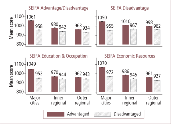
Notes: Sample sizes: Major cities advantaged n = 4,182; major cities disadvantaged n = 1,871; inner regional advantaged n = 1,299; inner regional disadvantaged n = 776; outer regional advantaged n = 919; outer regional disadvantaged n = 697. Differences in mean scores for remoteness × disadvantage, localities overall, disadvantage overall, and disadvantage within each locality were statistically significant (p < .05).
Source: LSAC Wave 1, B and K cohorts combined, linked Census data
Apart from major cities, it is notable that the differences by disadvantage and across geographic localities were more limited for the SEIFA Index of Education and Occupation. In a sense, this result is expected, as education and occupational status in particular areas are different from labour force participation.
3.3 Methods
Much of this report focuses on comparing the characteristics of families across the six socio-geographic areas:
- major city areas with low unemployment rates;
- major city areas with high unemployment rates;
- inner regional areas with low unemployment rates;
- inner regional areas with high unemployment rates;
- outer regional areas with low unemployment rates; and
- outer regional areas with high unemployment rates.
To make these comparisons, graphs showing means or percentages, with 95% confidence intervals or "I" bars, have been presented. In the graphs, non-overlapping confidence intervals in two columns suggest that we can be 95% confident that the two values represented in the columns are significantly different. However, overlapping confidence intervals does not necessarily suggest that the corresponding means or percentages are significantly different. Therefore, statistical tests were also conducted to assess whether differences in the figures were statistically significant.
Tests evaluated the significance of differences between: (a) the six socio-geographic areas (remoteness × disadvantage); (b) the three geographic localities overall; (c) disadvantaged and advantaged areas; and (d) disadvantaged and advantaged areas within each geographic locality. When the variable was a continuous measure, such as the SEIFA scores shown in Figure 2, t-tests were used to compare between disadvantaged and advantaged areas, and analysis of variance (ANOVA) was used to compare between the three types of geographic localities or between the six socio-geographic areas. When the variable was categorical, chi-square tests were used to assess the level of significance in differences across any of the groups. The results of these statistical tests are shown in the figure footnotes.
In Sections 4 to 9 of this report, various child and family characteristics are examined in relation to the socio-geographic areas described above. To present this information, we usually focus on characteristics as measured at one wave, combining the cohorts. While information is often available from multiple waves of LSAC, including data from more than one wave is not necessary to demonstrate the relationships. In fact, if more than one wave were used, more sophisticated methods would be required to assess the significance of differences across the six groups. As such, presentation of data from one wave proved to be the best approach. For some analyses, it was relevant to consider characteristics at different ages of children, and in those cases, more than one wave of data was used, but in doing so, these data were presented and analysed separately by the ages of the children. The sources of data are noted throughout the report. The specific characteristics examined are described in detail in each of the following sections.
Section 9 focuses on the children's learning, socio-emotional and physical outcomes; specifically whether children in regional areas experience a tyranny of distance or a tyranny of disadvantage in relation to these outcomes. Is it distance from major cities that explains the gaps in children's development in regional areas or is it mainly because these regional areas are often disadvantaged? As with other descriptive analyses, the various outcome measures are presented by the six socio-geographic areas. However, to formally test the statistical significance of differences between children living in advantaged and disadvantaged areas, and between the three geographic localities, we use multivariate analyses. These multivariate analyses also enable us to formally test whether any differences in children's outcomes according to disadvantage or distance can be explained by the different characteristics of the children and families in these areas. The measures used and the multivariate techniques applied are described in more detail in Section 9.
Footnotes
3 SLAs are based on the boundaries of incorporated bodies of local government, where these exist. SLAs are the smallest unit of geography for which statistical estimates can be calculated between Census years and therefore are most appropriate for use in longitudinal studies.
4 An alternative approach to classifying disadvantaged areas would have been to identify, at any wave, those regions with unemployment rates in the top 20% of the distribution. There are a few concerns with such an approach, which are best illustrated by a hypothetical example. Consider the example of area A, which is categorised as being disadvantaged in Wave 1 (i.e., it is in the top 20% of unemployment rate areas). By Wave 2, the unemployment rate for area A has increased further; however, the unemployment rates in other areas have increased even more than area A so that now, at Wave 2, even though the unemployment rate has increased in area A, it is no longer defined as being disadvantaged. In our preferred approach, area A would continue to be defined as being disadvantaged and the other areas that have had substantial increases in unemployment rates would also fall into this category.
4. Local area contextual factors
This section presents an overview of the different geographic localities within which the LSAC children live and comparing them according to their relative remoteness, as well as comparing areas that are disadvantaged to those that are not. First, we build a socio-demographic profile of the residents in these areas by using data linked to LSAC from the ABS Census of Population and Housing (the Census). In addition to these Census data on the socio-demographic profile of neighbourhoods, we present LSAC data on parent ratings on different aspects of the quality of their neighbourhood. More detailed demographic characteristics as captured in LSAC are then presented in Section 5.
A summary of the data analysed in this section is presented in Table 4.
| Measure | Values | Notes |
|---|---|---|
| Linked Census data (for SLA) | ||
| Economic resources | Percentage of persons completed Year 12 | Based on interpolation from 2001 and 2006 Census |
| Percentage of persons working (employed) | ||
| Percentage of persons with weekly income of < $1,000 | ||
| Cultural diversity | Percentage of persons who were Australia-born | Based on interpolation from 2001 and 2006 Census |
| Percentage of persons speaking only English at home | ||
| Percentage of persons with Aboriginal and Torres Strait Islander origins | ||
| Internet | Percentage of households with Internet capacity | Only available from 2006, so shown for Wave 2 (2006) |
| Percentage of households with broadband | ||
| LSAC data | ||
| Perceptions of neighbourhood (primary carers' ratings) | Agree or strongly agree that: | |
| Neighbourhood is safe | ||
| Neighbourhood is clean | ||
| Neighbourhood has good parks, playgrounds and play spaces | ||
| Neighbourhood has good roads, footpaths and lighting | ||
4.1 The demography of the area: Linked Census data
The linked Census data provide a broad view of the nature of the area within which the LSAC respondents live, and also provide information that is collected independently of LSAC, which is useful for building a picture of the area, as represented by those who are not parents of young children.
The linked Census data were derived from the two most recent Census periods, conducted in 2001 and 2006. As LSAC was conducted in 2004, 2006 and 2008, the 2004 and 2008 collections do not match these Census years; therefore, for 2004 and 2008, the characteristics from 2001 and 2006 were used to interpolate probable values for these years. Questions relating to Internet access were not asked in 2001, and so these data were not interpolated. (See the AIFS, 2011, LSAC Data User Guide, for more information about the linkage and interpolation process.)
These analyses present Census data for one wave of LSAC only, with Wave 1 being used for most data. Wave 2 data were used for Internet/broadband access, since these Census data were collected in 2006, around the time of the Wave 2 collection.
Figure 3 provides a comparison of some indicators of economic resources across the geographic localities and disadvantaged areas, using linked Census data.5 This figure shows, for the SLAs of each LSAC respondent, the percentage who had completed Year 12, the percentage in paid work and the percentage of families who had an income of less than $1,000 per week.
Figure 3: Area-level economic resources in Australian advantaged and disadvantaged areas, by geographic locality
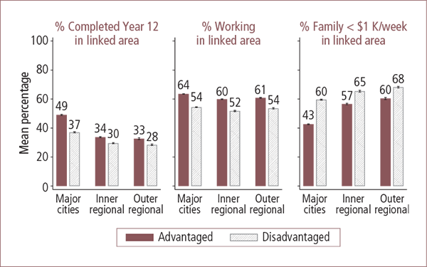
Notes: Sample sizes: Major cities advantaged n = 4,182; major cities disadvantaged n = 1,871; inner regional advantaged n = 1,299; inner regional disadvantaged n = 776; outer regional advantaged n = 919; outer regional disadvantaged n = 697. Differences in mean percentages for remoteness × disadvantage, localities overall, disadvantage overall, and disadvantage within each locality were statistically significant (p < .05).
Source: LSAC Wave 1, B and K cohorts combined, linked Census data
Compared to the other geographic localities, major city areas included a relatively high percentage of people who had completed a secondary education. This was especially so in advantaged areas in major cities (49%). Even in disadvantaged areas in major cities the percentage who completed their secondary education (37%) was relatively high compared to advantaged and disadvantaged inner and outer regional areas. Across all localities, the disadvantaged areas included a smaller percentage of the population who had completed secondary education than advantaged areas, with the lowest percentages being in disadvantaged inner and outer regional areas. Differences according to disadvantage, however, were not as great in the inner and outer regional areas as they were in major city areas.
Looking at the percentage of the population who were in paid work across the geographic localities, there was an expected difference in percentages according to whether or not the area was disadvantaged. Also, within advantaged areas, there was about a three-percentage point difference between geographic localities, with higher percentages being in paid work in major cities than in the inner or outer regional areas. Within disadvantaged areas, there was a higher percentage in paid work in major cities and outer regional areas compared to inner regional areas.
The percentage of families with incomes of less than $1,000 per week also varied across the geographic localities. Advantaged major city areas had the lowest percentage of families with lower incomes (43%), while the highest percentage of these families were living in disadvantaged inner (65%) and outer regional areas (68%). The differences in the percentages of lower income families were large, even between disadvantaged major city areas compared to disadvantaged inner and outer regional areas. In disadvantaged areas of major cities, 60% of families had an income of less than $1,000 per week, compared to 65-68% of families in disadvantaged inner and outer regional areas.
Cultural diversity is considered next. Figure 4 shows three indicators from the Census of ethnicity or cultural diversity across Australian localities. First, the percentage of Australian-born residents varied most in regard to the remoteness of the area, with much higher percentages of Australian-born people living in regional areas than in major cities. Within the regional areas, there was no apparent difference in the proportion of Australian-born residents according to the disadvantage of the area. Within major cities, however, a difference was apparent, with a somewhat smaller proportion of Australian-born people living in disadvantaged areas. These findings reflect migration patterns that see new arrivals to Australia being concentrated in disadvantaged areas of major cities (Hugo et al., 2010).
Figure 4: Cultural diversity in Australian advantaged and disadvantaged areas, by geographic locality
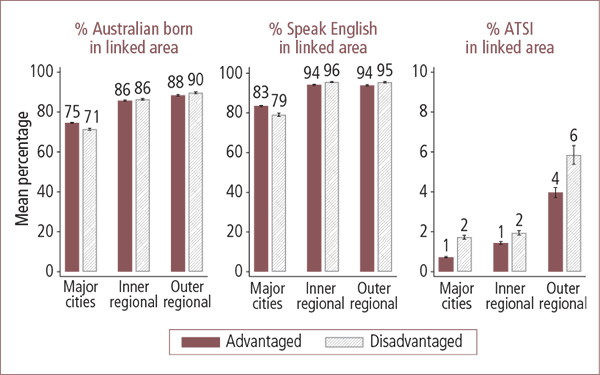
Notes: Sample sizes: Major cities advantaged n = 4,182; major cities disadvantaged n = 1,871; inner regional advantaged n = 1,299; inner regional disadvantaged n = 776; outer regional advantaged n = 919; outer regional disadvantaged n = 697. Differences between disadvantaged and advantaged areas in the percentages who were Australia-born were non-significant overall and within inner and outer regional areas (p > .05). All other differences in mean percentages for remoteness × disadvantage, localities overall, and disadvantage within major city areas were statistically significant (p < .05).
Source: LSAC Wave 1, B and K cohorts combined, linked Census data.
The proportions of people speaking only English at home presented a similar picture, with the vast majority of those living in areas of inner and outer regional Australia speaking only English. In major cities, while most people only spoke English, this proportion was lower than in regional areas, and especially so in disadvantaged parts of the major cities.
The proportion of the population who were Indigenous Australians within the LSAC respondents' localities was small overall, but Figure 4 shows that this proportion was highest in outer regional Australia, and was especially high in disadvantaged parts of those localities. We have not included remote parts of Australia here, where the percentage who were Aboriginal or Torres Strait Islander would have been significantly higher again (see Baxter et al., 2011).
Increasingly, the Internet is being used for service delivery (e.g., for banking) by both the government and private sectors. The proportion of the population having access to a reliable and fast Internet connection is therefore an important indicator of an area's level of access to services. Figure 5 indicates that both overall access to the Internet and access to broadband in particular show the same types of differences across geographic localities. The more remote the locality, the smaller the percentage of homes with access, and within localities, disadvantaged areas had a smaller percentage of homes with access.
Figure 5: Internet access in Australian advantaged and disadvantaged areas, by geographic locality

Notes: Sample sizes: Major cities advantaged n = 4,106; major cities disadvantaged n = 1,245; inner regional advantaged n = 1,180; inner regional disadvantaged n = 586; outer regional advantaged n = 848; outer regional disadvantaged n = 471. Differences in mean percentages for remoteness × disadvantage, localities overall, disadvantage overall, and disadvantage within each locality were statistically significant (p < .05).
Source: LSAC Wave 2, B and K cohorts combined, linked 2006 Census data
4.2 Parent reports on neighbourhood quality: LSAC data
In the LSAC survey, parents are asked to rate the quality of their neighbourhoods. In this section, we report on the primary carers' ratings of the degree to which they strongly agreed or agreed that their neighbourhood or local area: (a) was safe; (b) was clean; (c) had good parks, playgrounds and play spaces; and (d) had good roads, footpaths and lighting.
Figure 6 shows that, according to Wave 1 data, LSAC parents were quite positive about how safe and clean they perceived their neighbourhood to be. This was especially so for advantaged areas, but also for disadvantaged regional areas. Small differences in these measures were apparent across localities; most notably, significantly smaller percentages of parents living in disadvantaged areas in major cities and outer regional areas reported that their neighbourhood was safe and clean. For example, when comparing advantaged major city areas to disadvantaged major city areas, there was a seven percentage point difference in the proportion of parents agreeing that their neighbourhood was safe.
Figure 6: Perceptions of neighbourhood quality in Australian advantaged and disadvantaged areas, by geographic locality
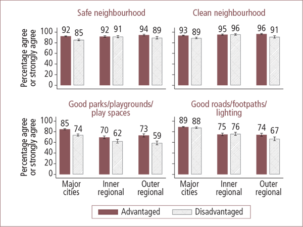
Notes: Sample sizes: Major cities advantaged n = 4,182; major cities disadvantaged n = 1,871; inner regional advantaged n = 1,299; inner regional disadvantaged n = 776; outer regional advantaged n = 919; outer regional disadvantaged n = 697. Differences by disadvantage were not significant (p > .05) for "safe neighbourhood" and "clean neighbourhood" in inner regional areas, and for "good roads, footpaths and lighting" in major cities and inner regional areas. All other differences in percentages for remoteness × disadvantage, localities overall, disadvantage overall, and disadvantage within each locality were statistically significant (p < .05).
Source: LSAC Wave 1, B and K cohorts combined
With regard to neighbourhood safety, the lack of differences between disadvantaged and advantaged inner regional areas may reflect the protective role that higher levels of social capital play in these communities. Certainly, work by Edwards and Bromfield (2009, 2010) showed that children living in socio-economically disadvantaged neighbourhoods with higher levels of social capital in the area had better social and emotional wellbeing than children living in disadvantaged neighbourhoods where social capital was lower. Other US studies have also reported similar findings; for example, in disadvantaged areas of Chicago, violent crime rates were lower when residents reported higher levels of social capital (Sampson, Raudenbush & Earls, 1997).
Parental perceptions of having access to good parks, playgrounds and play spaces varied between geographic localities and between disadvantaged and advantaged areas. When compared to parents living in advantaged areas, a significantly smaller percentage of parents living in the same locality but in disadvantaged areas reported that they had good parks, playgrounds and play spaces in their area. However, a greater percentage of parents living in disadvantaged major city areas reported having good play facilities than parents living in disadvantaged inner and outer regional areas. In advantaged areas, those most likely to agree that they had such facilities were those living in major cities, followed by those in outer then inner regional areas. For disadvantaged areas, there was a steady reduction in the percentage of parents who reported they had good play facilities from major cities through to inner, then outer regional areas. Only 59% of parents living in disadvantaged outer regional areas reported having good parks and playgrounds in their neighbourhood.
There were differences between advantaged and disadvantaged outer regional areas with respect to parents' perceptions about good roads, footpaths and lighting. A smaller percentage of parents living in a disadvantaged outer regional areas compared to advantaged outer regional areas reported good roads, footpaths and lighting. This finding may reflect inadequate infrastructure in more regional areas, particularly in the more disadvantaged areas.
Summary
This section has explored how local area characteristics vary for families living in different geographic localities of Australia. The clearest and most consistent findings were in regard to the differences between advantaged and disadvantaged areas. Disadvantaged areas, as defined by local area unemployment rates, were also characterised by disadvantage on measures of human capital and employment, as well as access to the Internet. Differences between disadvantaged and advantaged areas were particularly marked in major city areas. LSAC parents' reports on the quality of their neighbourhood also varied somewhat according to the disadvantage of the area, and this was most apparent with regard to having access to good parks, playgrounds and play spaces.
Some characteristics of local areas also varied according to the remoteness of the area, with higher levels of education and greater access to the Internet (and broadband) being evident among those living in major cities, and higher percentages of families having relatively low incomes in inner regional and outer regional areas. According to LSAC parents, the quality of the neighbourhood was not rated as highly in inner and outer regional areas, especially in terms of access to good parks, playgrounds and play spaces and having good roads, footpaths and lighting.
The cultural diversity and ethnicity of the geographic localities of Australia differed between major cities and regional areas with respect to the proportion of the population born overseas, speaking only English at home or being an Indigenous Australian. Not surprisingly, Indigenous Australians were a higher proportion of the population in outer regional areas than in inner regional areas or major cities. Within each type of locality, a higher percentage was Indigenous in disadvantaged rather than advantaged areas. Overseas-born and non-English speaking people made up higher proportions of the population in major cities than in the inner and outer regional areas, and in major cities, were somewhat more likely to be living in disadvantaged than advantaged areas.
These differences in demographic characteristics between advantaged and disadvantaged areas and between major city areas and regional areas may provide different opportunities for families and for children. The next sections now look more closely at family-level characteristics, and how they vary across these areas of Australia.
Footnote
5 These data were originally derived for each SLA across Australia, and have been matched to the LSAC data, according to the SLA within which a family lives. These matched Census data will therefore be the same for those respondents in the same area. The geographically clustered sample design of LSAC means that one SLA is likely to include a number of LSAC respondents, and so the variation in this matched data is diminished somewhat, and this is reflected in Figure 3 in the very narrow 95% confidence intervals.
5. Family demographic and economic characteristics
Turning now to the more immediate characteristics of the families within which children live, this section uses LSAC data to present some of the demographic and economic characteristics of families and parents across the different socio-geographic areas.
The measures explored here are described in Table 5.
| Measure | Values | Notes |
|---|---|---|
| Family form | Single-parent families Couple families | Couple-parent families are those with both a mother and father to the study child present in the household at the time of the study. If the study child has just one parent in the household in which they live at the time of the study, this family is categorised as a single-parent family. Some children may live in another household sometimes; for example, in shared care with a non-resident parent. These analyses do not consider to what extent this occurs. If another parent is only temporarily absent (for example, for work-related reasons), this family is classified as a couple-parent family. Families of different family forms (for example, headed by grandparents) are not shown in these analyses. |
| Mothers' country of birth and English-language proficiency | Mother born in Australia | |
| Mother born overseas, only English or good English-language proficiency | ||
| Mother born overseas, poor English-language proficiency | ||
| Parental education | Either parent (or single parent) has a bachelor degree or higher | The descriptive analyses show mothers' education levels in more detail. |
| Family joblessness | Jobless family (compared to at least one parent employed, not shown) | Indicates if single parent is not employed or if two couple parents are not employed. Those on long-term leave are included as jobless for these analyses. |
| Financial hardships | Number of financial hardships (0, 1, 2, 3+) | The primary carer was asked whether, over the previous 12 months, due to a shortage of money: (a) adults or children had gone without meals; (b) they were unable to heat or cool their home; (c) they had pawned or sold something; and/or (d) they had sought assistance from a welfare or community organisation. This is the count of how many of these hardships were reported. |
| Housing tenure | Own or buying house | |
| Renting or other tenure |
5.1 Family form
Figure 7 shows the percentage of LSAC families in each socio-geographic area who were couple or single parents. While most families were headed by couple parents, compared to advantaged areas, families in disadvantaged areas included a higher proportion headed by a single parent. This was true across all the geographic localities. Also, the families living in advantaged areas in major cities were less likely to be headed by single parents when compared with advantaged areas within inner and outer regional areas.
Figure 7: Family form in Australian advantaged and disadvantaged areas, by geographic locality

Notes: Sample sizes: Major cities advantaged n = 4,173; major cities disadvantaged n = 1,863; inner regional advantaged n = 1,297; inner regional disadvantaged n = 775; outer regional advantaged n = 913; outer regional disadvantaged n = 694. All differences in family form for remoteness × disadvantage, localities overall, disadvantage overall, and disadvantage within each locality were statistically significant (p < .05). Excludes other family forms such as those headed by grandparents.
Source: LSAC Wave 1, B and K cohorts combined
5.2 Mothers' place of birth and language proficiency
Differences in ethnicity that were apparent using the Census data were also apparent in the LSAC sample (Figure 8). The vast majority of mothers in inner and outer regional areas were Australian-born, and if born overseas, had good English-language proficiency or spoke only English. There was more diversity in major cities, with a significant proportion being overseas-born but with good English language proficiency or speaking only English (29% in advantaged and 27% in disadvantaged areas). In major cities, 4% of mothers in advantaged areas and 6% in disadvantaged areas had poor English-language proficiency. Future analyses of these data could explore in more detail the countries of birth of these mothers, and also their migration history.6
Figure 8: Maternal country of birth and English-language proficiency in Australian advantaged and disadvantaged areas, by geographic locality
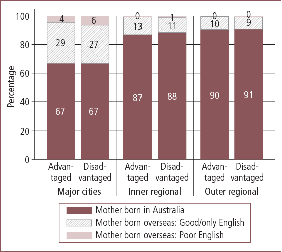
Notes: Sample sizes: Major cities advantaged n = 4,182; major cities disadvantaged n = 1,871; inner regional advantaged n = 1,299; inner regional disadvantaged n = 776; outer regional advantaged n = 919; outer regional disadvantaged n = 697. Differences in country of birth/English-language proficiency were non-significant (p > .05) when comparing by disadvantage within inner and outer regional areas. All other differences for remoteness × disadvantage, localities overall, disadvantage overall, and disadvantage within major city areas were statistically significant (p < .05).
Source: LSAC Wave 1, B and K cohorts combined.
5.3 Parental education
Parental education levels have broad implications for children, being linked to the employment and incomes of parents, as well as different approaches to parenting. Most studies of children's development have found that higher levels of maternal education are related to better social and behavioural development and are even more influential for children's cognitive outcomes (Dearing, McCartney, & Taylor, 2001; Jackson, Brooks-Gunn, Huang, & Glassman, 2000; McLeod & Shanahan, 1993). Therefore, maternal education is an important demographic variable to examine, and the findings from this study are shown in Figure 9.
Figure 9: Maternal educational attainment in Australian advantaged and disadvantaged areas, by geographic locality

Notes: Sample sizes: Major cities advantaged n = 4,170; major cities disadvantaged n = 1,860; inner regional advantaged n = 1,292; inner regional disadvantaged n = 770; outer regional advantaged n = 915; outer regional disadvantaged n = 689. Differences in parental education distribution were non-significant (p > .05) when comparing disadvantaged to advantaged inner regional areas. All other differences for remoteness × disadvantage, localities overall, disadvantage overall, and disadvantage within major city and outer regional areas were statistically significant (p < .05).
Source: LSAC Wave 1, B and K cohorts combined
The more remote and disadvantaged the area, the less likely mothers were to have a university qualification, and more likely to have an incomplete secondary education. For example, 31% of mothers in advantaged major city areas had a university degree, while 17% or fewer had a university degree in the five other areas. The percentage of mothers with a university qualification was lowest in disadvantaged outer regional areas, at 11%. We return to examine the educational activities that parents provide for children in Section 8.
5.4 Employment and economic status
Next, parental employment is examined by considering the percentage of families in which no parent was employed; that is, the incidence of family joblessness. Parental employment provides important financial resources for families, and children in jobless families are at greater risk of experiencing poorer outcomes (Gray & Baxter, 2011; Taylor, Edwards, & Gray, 2010).
Figure 10 shows that the highest rates of joblessness in families were in disadvantaged areas - 19% of children in disadvantaged areas of major cities were living with jobless parents at Wave 1 of LSAC, as were 17% of those in inner regional areas and 21% of those in outer regional areas. Not surprisingly, given the definition of disadvantaged is based on unemployment rates, family jobless figures were considerably lower in advantaged areas, at 9% in advantaged areas of major cities and 11% in inner and outer regional areas.
Figure 10: Family joblessness in Australian advantaged and disadvantaged areas, by geographic locality
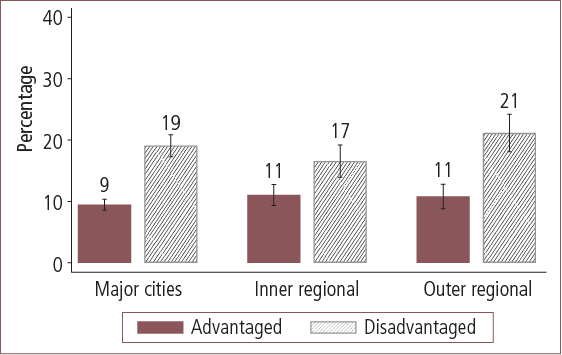
Notes: Sample sizes: Major cities advantaged n = 4,177; major cities disadvantaged n = 1,866; inner regional advantaged n = 1,298; inner regional disadvantaged n = 775; outer regional advantaged n = 915; outer regional disadvantaged n = 695. All differences in the percentage of jobless families for remoteness × disadvantage, localities overall, disadvantage overall, and disadvantage within each locality were statistically significant (p < .05).
Source: LSAC Wave 1, B and K cohorts combined
The higher incidence of lone parents and joblessness in disadvantaged areas, especially in major cities, leads to an expectation that financial wellbeing may be more difficult for families to achieve in these areas. One measure of financial wellbeing is families' experiences of financial hardships, as shown in Figure 11. This is measured as the number of financial hardships families had experienced in the previous twelve months. In LSAC, the primary carer was asked whether, over the previous 12 months, due to a shortage of money adults or children: (a) had gone without meals; (b) were unable to heat or cool their home; (c) had pawned or sold something; and/or (d) had sought assistance from a welfare or community organisation. Here we report on how many of these hardships were reported.7
Figure 11: Experiences of hardship by families in Australian advantaged and disadvantaged areas, by geographic locality
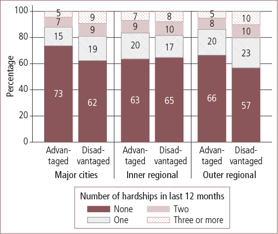
Notes: Sample sizes: Major cities advantaged n = 4,174; major cities disadvantaged n = 1,865; inner regional advantaged n = 1,296; inner regional disadvantaged n = 774; outer regional advantaged n = 919; outer regional disadvantaged n = 692. Differences in the distribution of hardships were non-significant (p > .05) when comparing disadvantaged to advantaged inner regional areas. All other differences for remoteness × disadvantage, localities overall; disadvantage overall, and disadvantage within major city and outer regional areas were statistically significant (p < .05).
Source: LSAC Wave 1, B and K cohorts combined
These data, using Wave 1 of LSAC, confirm that families in disadvantaged major city areas had a higher incidence of hardships compared to families in advantaged major city areas. Families in advantaged areas of major cities were the least likely to report any hardships. Within inner regional areas, the experiences of financial hardship did not appear to vary according to the disadvantage of the area. However, within outer regional areas, families were more likely to experience financial hardships if they lived in a disadvantaged area. This group experienced the highest rates of financial hardships.
Figure 12 describes families' housing tenure in the six socio-geographic areas, at Wave 1. Although there is a large difference in the percentage of families owning or buying their house in advantaged areas compared to disadvantaged areas in major cities (70% compared to 58%), these differences were much smaller for inner regional (69% compared to 63%) and outer regional areas (64% compared to 56%). The greater affordability of housing outside of the major cities may be one of the reasons for these smaller differences between families residing in advantaged and disadvantaged inner and outer regional areas. In fact, other research is consistent with these findings, with McNamara, Tanton and Phillips (2007) reporting that housing stress appeared to be greatest on the fringes of the major cities, but not in inner regional and outer regional areas. The affordability of housing in inner regional areas may also be the reason for the similar rates of financial hardship in inner regional areas.
Figure 12: Housing tenure in Australian advantaged and disadvantaged areas, by geographic locality

Notes: Sample sizes: Major cities advantaged n = 4,177; major cities disadvantaged n = 1,866; inner regional advantaged n = 1,299; inner regional disadvantaged n = 774; outer regional advantaged n = 918; outer regional disadvantaged n = 695. All differences in housing tenure for remoteness × disadvantage, localities overall, disadvantage overall, and disadvantage within each locality were statistically significant (p < .05).
Source: LSAC Wave 1, B and K cohorts combined
5.5 Summary
The family demographic and economic contexts for children's development are quite different in regional areas when compared to the major cities. But with regard to many of these characteristics, it was advantaged areas in major cities that stood apart from the other areas examined. Compared to other areas of Australia, in advantaged major city areas there was a higher proportion of children living with a mother with university education, with couple parents, with employed parents, in a home that was owned or being purchased, and in families who had experienced no financial hardships in the past year. On all these indicators, children in disadvantaged areas of major cities were living in more unfavourable circumstances. Similarly, conditions for the families in inner and outer regional areas of Australia, even if living in advantaged areas, were more unfavourable compared to those living in advantaged major city areas.
Advantaged inner and outer regional areas were often very similar to each other with regard to family demographic and economic characteristics. However, some differences were apparent when comparing these areas to disadvantaged inner regional and outer regional areas. In disadvantaged (inner and outer) regional areas, there were higher percentages of single-parent families, jobless families and families who were renting, compared to their advantaged counterparts. In disadvantaged outer regional areas, there were higher percentages of mothers with relatively low educational attainment and families experiencing financial hardships, compared to advantaged outer regional areas.
Consistent with the local area data presented in the previous section, most mothers in inner and outer regional areas were Australian-born, and if born overseas, spoke English well. Major city areas were more diverse, with higher proportions born overseas, although the majority had good English-language proficiency or only spoke English. Within the major city areas, somewhat more mothers in disadvantaged, compared to advantaged, areas were born overseas and had poor English-language proficiency.
Footnotes
6 Of overseas-born mothers, about 67% of those with poor English-language skills had arrived after 1994, compared with 37% of those who spoke only English or good English.
7 Additional questions (not used here) were asked about being able to pay gas, electricity or telephone bills on time, and being able to pay the mortgage or rent on time, which are related more to having cash flow problems than experiencing hardships. We have focused on the hardship questions based on Bray's (2001) distinction between cash flow and hardship problems. Moreover, according to the literature, the adverse experience of hardship is particularly detrimental to family functioning and this is more closely tied to hardship and missing out than to cash flow problems (Conger & Elder, 2001).
6. Parent wellbeing and parenting style
Contexts for children's social development include the immediate family environment, especially parents' wellbeing and parenting style. In this section, we examine parental wellbeing as, according to the family stress model (Elder & Conger, 2000) and the empirical literature, if parents suffer from mental health problems, this can impair their ability to parent and be responsive to their child's needs, and may be associated with more irritable and angry parenting and lower parental warmth (Kane & Garber, 2004; Lovejoy, Gracyzk, O'Hare & Neuman, 2000; Wilson & Durbin, 2010). Conflict in the parental relationship (Conger & Elder, 1994; Elder & Conger, 2000) and high levels of alcohol consumption (Dawe et al., 2007) also affect the ability to parent effectively. Parental levels of being overweight or obese also reflect diet in the home and family levels of physical activity (Harrison et al., 2011).
The measures explored here are described in Table 6.
| Measure | Values | Notes |
|---|---|---|
| Parent wellbeing | ||
| Parent mental health | Serious mental health risk (compared to those with no serious mental health risk, not shown) | Based on Kessler 6 scale, those with a score of 13 or more (on a scale of 0 to 24) are coded as being at risk of serious mental health problems. See also footnote 7. |
| Parental relationships | Parental relationship is often hostile (compared to those whose relationship is not hostile, not shown) | "Often hostile" includes those who have reported that there are often or always arguments, often or always hostility, or often or always violence in their relationship. |
| Parental drinking habits | Mother binge drinking Father binge drinking | Derived from parents' reports of how often they binge drink. Binge drinking is defined as 7 or more (men) and 5 or more (women) drinks on an occasion, at least 2-3 times a month. The multivariate analyses include an indicator of parents' binge drinking and for parents abstaining from alcohol. Parental binge drinking was compared to parental light/moderate drinking. |
| Parental weight status | Overweight, including overweight, obese class 1 or 2, or extreme obesity, (compared with underweight or normal weight, not shown) | Based on parents' body mass index (BMI) scores. Mothers' and fathers' weight status shown separately. |
| Parenting style | ||
| Warm parenting | Relatively low parental warmth (compared to those who did not have relatively low parental warmth, not shown) | This is derived from the LSAC parental warmth scale. Within each cohort and wave, the distribution of this scale was evaluated, and those who fell in the bottom 20% of the scale were identified. Mothers' and fathers' warmth were analysed separately, and for multivariate analyses an indicator of either parent having low parenting warmth was used. |
| Angry parenting | Relatively high angry parenting (compared to those who did not have relatively high angry parenting, not shown) | This is derived from the LSAC angry parenting scale. Within each cohort and wave, the distribution of this scale was evaluated, and those who fell in the top 20% of the scale were identified. Mothers' and fathers' angry parenting were analysed separately, and for multivariate analyses, an indicator of either parent having high angry parenting was used. |
6.1 Parent wellbeing
Parent mental health
As argued previously, the research literature suggests that the wellbeing of mothers and fathers is important for their children's own wellbeing. One indicator of parental wellbeing is mental health. Parental mental health problems are measured in LSAC using the Kessler 6 (K6) scale. It comprises six items and has been widely used and validated in many epidemiological studies (e.g., Kessler et al., 2002). Parents who score highly on this measure are considered to be at risk of a serious mental illness (other than a substance use disorder).8 It is important to recognise that the K6 screens for the risk of serious mental illness and is not a diagnostic measure. The percentage of mothers and fathers who were at risk of mental health problems was low, at around 3% of mothers and fewer than 2% of fathers, and there were no statistically significant differences between socio-geographic areas for mothers and fathers.
Parental relationships
The quality of parents' relationships with each other is also an important factor in regard to children's wellbeing. Mothers' and fathers' reports of the quality of their relationship were used to derive an indicator of couples who are often or always hostile. This includes those who reported that there were often or always arguments, hostility or violence in their relationship. Fewer than 10% of mothers and fathers reported that their relationship was always or often hostile. There were no statistically significant differences in the presence of hostile relationships between geographic localities or between disadvantaged and advantaged areas.
Parental drinking habits
Figure 13 shows the degree to which parents in advantaged and disadvantaged areas undertook binge drinking. The 2001 National Health and Medical Research Council (NHMRC; 2003) guidelines for risky binge drinking was used to guide the development of the measure of binge drinking in LSAC. Binge drinking is defined as 7 or more (for men) or 5 or more (for women) standard drinks on one occasion two to three times a month or more (Dawe et al., 2007).
Figure 13: Incidence of binge drinking among mothers and fathers in Australian advantaged and disadvantaged areas, by geographic locality
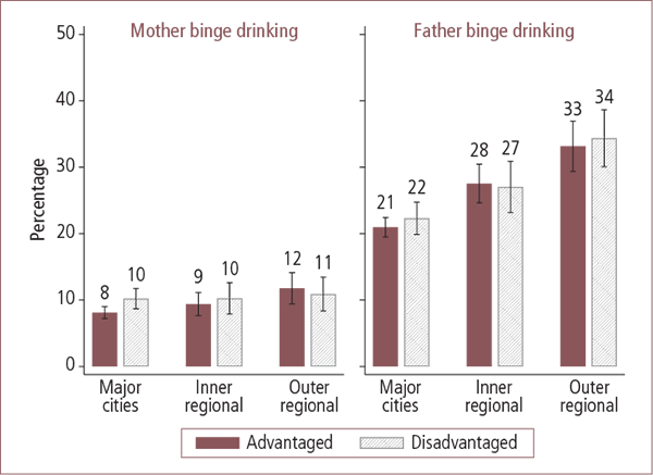
Notes: Sample sizes: Major cities advantaged n = 3,454, major cities disadvantaged n = 1,502; inner regional advantaged n = 1,098; inner regional disadvantaged n = 634; outer regional advantaged n = 723; outer regional disadvantaged n = 577. For fathers, sample sizes are lower, with the lowest being 476 in disadvantaged outer regional areas. For mothers, all differences for remoteness × disadvantage, localities overall, disadvantage overall, and disadvantage within each locality were not statistically significant (p > .05). For fathers, differences for disadvantage overall and disadvantage within each locality were not significant, but differences were significant for localities overall (p < .05).
Source: LSAC Wave 1, B and K cohorts combined
For fathers, very large and statistically significant differences in their drinking habits were apparent between regional areas, but not by whether they lived in disadvantaged or advantaged areas. Fathers living in disadvantaged outer regional areas had the highest rates of binge drinking (34%), compared to fathers living in advantaged major city areas (21%). Binge drinking was also much higher in inner regional areas (27-28%). Rates of binge drinking were much lower for mothers than they were for fathers, and did not have the same geographic variation that was evident for fathers.
Parental weight status
Parents being overweight or obese reflects dietary choices in the home and levels of physical activity, which can, in turn, influence children's chances of being overweight or obese (Harrison et al., 2011). There is also a genetic component to childhood overweight and obesity, with studies estimating that up to 77% of variation in body mass index is inherited (Beyerlein, von Kries, Ness, & Ong, 2011; Wardle, Carnell, Haworth, & Plomin, 2008).
Figure 14 shows the percentage of mothers and fathers of LSAC children who were overweight or obese. Based on their body mass index (BMI), the majority of parents were classified as overweight, obese class 1 or 2, or extremely obese, as opposed to underweight or normal weight. For mothers, being overweight or obese ranged from 39% to 51%, and for fathers 64% to 73%. Differences between geographic localities and between disadvantaged and advantaged areas were apparent. For mothers, a higher proportion was overweight in regional areas and in disadvantaged areas, with the highest percentage overweight living in disadvantaged outer regional areas. The difference in the percentage overweight between disadvantaged and advantaged areas of major cities was statistically significant. For fathers, there was a relatively high percentage overweight or obese in inner regional areas. In outer regional areas, it was in the advantaged rather than the disadvantaged areas that a higher percentage of fathers were overweight.9
Figure 14: Overweight status among mothers and fathers in Australian advantaged and disadvantaged areas, by geographic locality
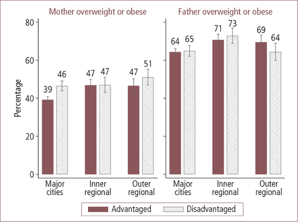
Notes: Sample sizes: For mothers, major cities advantaged (n = 3,330); major cities disadvantaged (n = 1,421); inner regional advantaged (n = 1,066); inner regional disadvantaged (n = 610); outer regional advantaged (n = 688); outer regional disadvantaged (n = 543). Sample sizes for fathers were somewhat lower, with the lowest being 440 for outer regional disadvantaged. For mothers, differences in percentages were significant for remoteness × disadvantage, localities overall, disadvantage overall, and disadvantage within major cities. For fathers, differences in percentages were significant for remoteness × disadvantage, locality, and disadvantage within outer regional areas.
Source: LSAC Wave 1, B and K cohorts combined
6.2 Parenting style
Parenting style has been found to have strong links with children's outcomes. An authoritative parenting style - where parents exert firm control, engage in calm discussions with their children and are warm and affectionate - has been associated with enhanced cognitive skills and fewer behaviour problems in children (Linver, Brooks-Gunn, & Kohen, 2002; Pettit, Bates, & Dodge, 1997). Angry, coercive parenting that is lacking in affection has been linked to more problematic outcomes (Edwards, Baxter, Smart, Sanson, & Hayes, 2009; Smart, Sanson, Baxter, Edwards, & Hayes, 2008). In this section, we use two variables that indicate the more problematic parenting styles described above: lower parental warmth and higher angry parenting. These items have been presented just for the K cohort (at Wave 1), since the measure of angry parenting is not available for the B cohort at Waves 1 and 2. A description of these parenting variables follows.
Parental warmth was measured by asking parents about how often they displayed warm affectionate behaviour towards their child; for example, "How often do you enjoy doing things with this child?" and "How often do you express affection by hugging, kissing and holding this child?" The nature of the specific questions differed somewhat to reflect the age of the child, and parents were asked to rate the extent to which warmth was displayed, ranging from "never/almost never" to "always/almost always". Scores were then summed, and those falling into the lowest quintile (fifth) were classified as indicating lower warmth. It should be noted that parents generally gave positive answers to these questions (usually in the "often" or "always/almost always" range), and hence a position in the lowest quintile does not indicate very low warmth; rather that those scores were lower than the remainder of the sample.
Angry parenting was evaluated by asking parents about the extent to which they engaged in irritable and angry behaviours. Items contributing to this measure included parents' self-reports on how often their talking with children involved praise or disapproval, and about different aspects of their being angry with or punishing their child. Parents responded to these by indicating that they did this from "never/almost never" to "all the time". Scores on these items were summed and those in the upper quintile (the highest fifth of scores) were classified as indicating higher angry parenting. Parents generally did not report much angry parenting, hence this classification indicates relatively high but not very high levels of angry parenting.
The percentage of mothers with lower parental warmth who were living in advantaged and disadvantaged major city, inner regional and outer regional areas ranged from 16% to 23%. Differences between areas were not statistically significant but, overall, a smaller percentage of mothers had lower warm parenting in disadvantaged areas. There were no statistically significant differences between geographic localities or between disadvantaged and advantaged areas for fathers (Figure 15).
Figure 15: Mothers and fathers with lower warm parenting styles in Australian advantaged and disadvantaged areas, by geographic locality

Notes: Sample sizes: Major cities advantaged n = 2,064; major cities disadvantaged n = 852; inner regional advantaged n = 618; inner regional disadvantaged n = 384; outer regional advantaged n = 473; outer regional disadvantaged n = 342. Sample sizes for fathers were slightly lower, with the smallest being 242 for disadvantaged outer regional areas. Differences for mothers' warm parenting were non-significant for remoteness × disadvantage, localities overall, and disadvantage within each locality, but were significantly different for disadvantage overall. Fathers' warm parenting did not vary significantly for remoteness × disadvantage, localities overall, disadvantage overall, or disadvantage within each locality.
Source: LSAC Wave 1, K cohort
Looking at the proportions of parents with higher angry parenting (Figure 16), the only statistically significant variation was between geographic localities for mothers; a somewhat smaller percentage of mothers had higher angry parenting in inner regional areas compared with the other localities.
Figure 16: Mothers and fathers with higher angry parenting styles in Australian advantaged and disadvantaged areas, by geographic locality
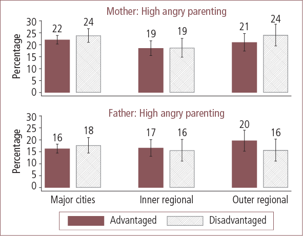
Notes: Sample sizes: Major cities advantaged n = 2,063; major cities disadvantaged n = 852; inner regional advantaged n = 618; inner regional disadvantaged n = 384; outer regional advantaged n = 473; outer regional disadvantaged n = 342. Sample sizes for fathers were slightly lower, with the smallest being 242 for disadvantaged outer regional areas. Differences for mothers' angry parenting were non-significant for remoteness × disadvantage, disadvantage overall, and disadvantage within each locality, but were significantly different for localities overall. Fathers' angry parenting did not vary significantly for remoteness × disadvantage, localities overall, disadvantage overall, or disadvantage within each locality.
Source: LSAC Wave 1, B and K cohort
6.3 Summary
Overall, this section presents quite mixed findings with regard to how parent wellbeing and parenting styles differ between geographic localities and between disadvantaged and advantaged areas. There were no differences between rates of parental mental health problems and parental relationship hostility between geographic localities and areas categorised as disadvantaged or advantaged based on unemployment rates. There was also little difference in the parenting styles of mothers and fathers, although these analyses found that mothers were somewhat more likely to have a relatively high angry parenting style in inner regional areas compared to other areas, and somewhat more likely to have a lower warm parenting style in disadvantaged rather than advantaged areas.
There were considerable locality differences in the level of binge drinking of fathers. One in three fathers engaged in binge drinking in outer regional areas compared to one in five in major city areas. For mothers, the differences between localities were not evident for this variable.
A complex pattern of differences for mothers being overweight or obese was evident between geographic localities and advantaged and disadvantaged areas. Mothers living in advantaged major city areas had the lowest rates of being overweight or obese when compared to the other five socio-geographic areas. Mothers living in disadvantaged regional areas had the highest levels compared to the other five areas. Mothers living in disadvantaged major city areas, inner regional areas (advantaged and disadvantaged) and advantaged outer regional areas all had very similar levels of being overweight or obese. Among fathers, the highest levels of being overweight were in inner regional areas, and higher proportions were overweight in advantaged compared to disadvantaged outer regional areas.
Footnotes
8 The K6 questions ask the respondent how often in the last four weeks they felt: (a) nervous; (b) hopeless; (c) restless or fidgety; (d) so depressed that nothing could cheer you up; (e) that everything was an effort; and (f) worthless. There were five response categories, from "none of the time" to "all the time", with values of 0 through to 4. These values were summed, and those with a sum of 13 or higher, out of a possible maximum of 24, were said to be at serious risk of having mental health problems.
9 This difference was statistically significant as indicated by a chi-square test, but not when using confidence intervals. As these statistical tests are reliant on different assumptions but are not consistent, caution should be used when interpreting this finding.
7. Family social capital and access to services
Social capital is considered next. In the context of the neighbourhood, social capital can be understood as the social connections between people in the neighbourhood that encourage trust, support and a shared understanding (Stone, 2001). This section also focuses on measures of the ability of family and friends to provide support and involvement in volunteer organisations. These have been found in other studies to be important in the positive development of children (e.g., Elder & Conger, 2000). Sometimes, if informal supports are not available, these can be offset by the provision of formal services; so we also examine the extent to which families experience difficulties in accessing such services.
Table 7 describes the measures explored in more detail.
| Measure | Values | Notes |
|---|---|---|
| Help from family and friends | Does not get enough help from family and friends (compared to those who do get enough help or who do not need help, not shown) | Derived from a question asking "Overall, how do you feel about the amount of support or help you get from family or friends living elsewhere?" Includes those who selected "I don't get enough help" or "I don't get any help at all", as opposed to "I get enough help" or "I don't need any help". This item was only available for Wave 1, B and K cohorts. |
| Unmet demand for support | Has unmet demand for support or help (compared to those who do not, not shown) | Derived from the question "How often do you feel that you need support or help but can't get it from anyone?" Includes those who said "very often" or "often", as opposed to "sometimes", "never" or "I don't need it". Those who had, in a previous question (above), said they do not need any help were coded as not having an unmet demand for support or help. |
| Contact with family, friends or neighbours | Weekly or daily contact with family, friends or neighbours (compared to less frequent contact) | Derived from questions asking about frequency of contact (how often you see, talk or email) with family, friends or neighbours. A separate indicator was examined for each of family, friends and neighbours. |
| Involvement in volunteer or community groups | Involved in volunteer groups (compared to those not involved, not shown) | The question used to derive this item varied across waves/cohorts. B cohort, Waves 1 and 2, parents were asked "Are you involved with any of these types of groups or organisations in a voluntary (unpaid) capacity? (This can be as a participant or voluntary worker/office bearer.)", with a list of 14 groups/organisations. B cohort, Wave 3, and K cohort, Waves 1 to 3, parents were asked "Do you participate in any ongoing community service activity (e.g., volunteering at a school, coaching a sports team or working with a church or neighbourhood association)?" |
| Neighbourhood belonging | Low neighbourhood belonging (compared to those who do not have low neighbourhood belonging, not shown) | Uses neighbourhood belonging scale, which is based on LSAC items assessing parents' trust of neighbours, sense of identity with the neighbourhood, how well-informed they are about local affairs, and knowledge about where to find information about local services. Those with low neighbourhood belonging were those with scores between 2.7 and 5, on a 1 to 5 scale in which higher scores reflected lower neighbourhood belonging. This represented 28% of the sample. |
| Services use | Child used one or more service in previous 12 months | Derived from responses to a question asking about whether, in the previous 12 months, the study child had used any of a list of community services. a |
| Family used one or more service in previous 12 months | Derived from responses to a question asking about whether, in the previous 12 months, anyone in the family had used any of a list of community services. | |
| Unmet demand for services | Unmet demand for services for child in previous 12 months | Derived from responses to question asking whether any of the services listed were needed but could not be accessed. |
| Unmet demand for services for family in previous 12 months | Derived from responses to question asking whether any of the services listed were needed but could not be accessed. |
Notes: a For B cohort, Wave 1, for example, the list of services was: (a) playgroup or parent-child group; (b) maternal and child health centre/phone help; (c) maternal and child health nurse visits; (d) paediatrician; (e) other specialist; (f) hospital emergency ward; (g) hospital outpatients clinic; (h) GPs; (i) other medical or dental services; and (k) other child-specific services. The list for the K cohort was similar, but included early education services, speech therapy, guidance counsellors and other psychiatric or behavioural services.
7.1 Social capital
Looking now beyond the family environment, in this section we explore some measures of connections with broader family, friends and the community. These analyses are based on the reports of the child's primary carer.
Figure 17 shows the proportion of parents who, in Wave 1, reported that they very often or often needed support but could not get it, and the proportion who reported that they do not get enough help from family or friends. Differences in unmet need for support were not apparent between geographic localities or between disadvantaged and advantaged areas. However, reporting to have not received enough or any help from family and friends was more likely in major cities than in inner or outer regional areas. Within major city areas, those living in advantaged areas were more likely than those living in disadvantaged areas to say that they had not received enough or any help from family and friends. This difference was not apparent in inner and outer regional areas.
Figure 17: Unmet need for support and not enough help from family and friends in Australian advantaged and disadvantaged areas, by geographic locality
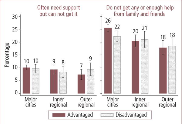
Notes: Sample sizes for needing support: Major cities advantaged (n = 3,317); major cities disadvantaged (n = 1,446); inner regional advantaged (n = 1,063); inner regional disadvantaged (n = 614); outer regional advantaged (n = 679); outer regional disadvantaged (n = 559). Sample sizes were somewhat higher for not enough help from family and friends. For needing support, differences for remoteness × disadvantage, localities overall and disadvantage overall were not statistically significant. For not enough help from family and friends, differences for remoteness × disadvantage, localities overall, disadvantage overall, and disadvantage in major cities were significant.
Source: LSAC Waves 1, B and K cohorts
More than nine in ten parents (primary carers) had daily or weekly contact with family members, and around three-quarters of parents had weekly or daily contact with friends. There were no statistically significant differences in these percentages between geographic localities or between disadvantaged and advantaged areas. Regular contact with neighbours was less common than with family members, with around half the parents saying they had weekly or daily contact with their neighbours. Again, there was no statistically significant variation by socio-geographic area (results not shown).
One commonly used measure of social capital is parental involvement in volunteer groups or organisations (Elder & Conger, 2000; Leigh, 2010). B cohort parents were asked: "Are you involved with any of these types of groups or organisations in a voluntary (unpaid) capacity? (This can be as a participant or voluntary worker/office bearer.)", and given a list of 14 groups/organisations. K cohort parents were asked: "Do you participate in any ongoing community service activity (e.g., volunteering at a school, coaching a sports team or working with a church or neighbourhood association)?" Figure 18 shows that involvement was somewhat more common in areas that were advantaged than in disadvantaged areas. In advantaged areas, involvement was higher in inner regional areas compared to major cities, and higher again in outer regional areas. Gaps in parental involvement between advantaged and disadvantaged areas were greatest in outer regional areas, followed by major city areas and then inner regional areas.
Figure 18: Parental involvement in community groups or organisations in Australian advantaged and disadvantaged areas, by geographic locality

Notes: Sample sizes: Major cities advantaged (n = 3,469); major cities disadvantaged (n = 1,478); inner regional advantaged (n = 1,100); inner regional disadvantaged (n = 636); outer regional advantaged (n = 730); outer regional disadvantaged (n = 591). Differences for remoteness × disadvantage, localities overall and disadvantage overall were all statistically significant, except between disadvantaged and advantaged inner regional areas (p < .05).
Source: LSAC Wave 1, B and K cohorts combined
In Wave 1, LSAC parents also reported on the types of volunteer groups or organisations with which they were involved. According to these data, the most commonly reported volunteer groups or organisations, across localities, were playgroups, preschools and schools; sport or recreation groups; and religious groups. Figure 19 shows parental involvement in playgroups, preschools or schools was considerably lower in disadvantaged compared to advantaged areas, overall and within geographic localities. Also, participation in these groups was more likely in regional than in major city areas, with the highest participation rates being in outer regional areas.
Figure 19: Participation by parents in most commonly reported voluntary organisations in Australian advantaged and disadvantaged areas, by geographic locality
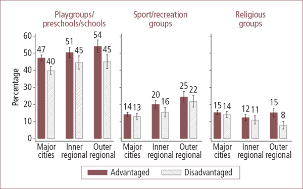
Notes: Percentages are calculated over all people, including those who were non-participants in voluntary activities. Sample sizes: Major cities advantaged (n = 3,469); major cities disadvantaged (n = 1,478); inner regional advantaged (n = 1,100); inner regional disadvantaged (n = 636); outer regional advantaged (n = 730); outer regional disadvantaged (n = 591). Differences for remoteness × disadvantage, localities overall and disadvantage overall were all significant for playgroups, preschools and schools. Sport/recreation groups varied for remoteness × disadvantage, localities overall, and disadvantage within inner regional areas. Religious groups varied for remoteness × disadvantage, localities overall, disadvantage overall and disadvantage within outer regional areas.
Source: LSAC Wave 1, B and K cohorts combined
Perhaps reflecting a greater emphasis on sport in rural areas, there were higher rates of participation by parents in sport or recreation groups in regional compared to major city areas, particularly in outer regional areas. There were no significant differences between disadvantaged and advantaged areas within major cities and outer regional areas, although overall, participation in these groups was more likely in advantaged areas.
Although only about one in eight families were involved in religious groups, families living in advantaged outer regional areas had significantly higher rates of participation in religious groups than families living in disadvantaged outer regional areas.
The primary measure of neighbourhood social capital in LSAC is neighbourhood belonging. Neighbourhood belonging assesses parents' trust of neighbours, sense of identity with the neighbourhood, degree of being well-informed about local affairs, and knowledge about where to find information about local services (see Edwards, 2006, for further information). It has been found to play an important role in explaining the differences in 4-5 year old children's social and emotional wellbeing when living in socio-economically disadvantaged compared to advantaged neighbourhoods (Edwards & Bromfield, 2009, 2010). In this study, those falling into the lowest quintile of scores on neighbourhood belonging were classified as having low neighbourhood belonging.
Figure 20 shows that lower neighbourhood belonging varies according to geographic locality, and differs for disadvantaged and advantaged areas. Lower neighbourhood belonging was most likely in disadvantaged major city areas (36%), compared to the other five socio-geographic areas. There were statistically significant differences between disadvantaged and advantaged areas overall and within major city areas, with lower belonging in disadvantaged areas. Differences between geographic localities were also apparent, with smaller percentages reporting relatively low neighbourhood belonging in outer regional areas, compared to inner regional and major city areas.
Figure 20: Lower neighbourhood belonging in Australian advantaged and disadvantaged areas, by geographic locality
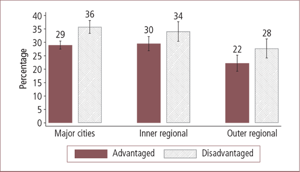
Notes: Sample sizes: Major cities advantaged (n = 3,543); major cities disadvantaged (n = 1,533); inner regional advantaged (n = 1,139); inner regional disadvantaged (n = 654); outer regional advantaged (n = 743); outer regional disadvantaged (n = 607). Differences for remoteness × disadvantage, localities overall, disadvantage overall, and disadvantage within major cities were statistically significant (p < .05).
Source: LSAC Waves 1, B and K cohorts combined
7.2 Service use and access to services
Discussions around the tyranny of distance of living in rural areas often centre around the ability of residents to access services. The definition of inner regional and outer regional areas is based on road distances from major service centres, and we therefore expected to find lower levels of service use in these regional areas. However, Figure 21 shows that very high rates of service use were reported for children in the last 12 months regardless of the area of residence. The only significant difference apparent in these data is that children living in major cities were somewhat less likely to use a service if they were living in a disadvantaged rather than an advantaged area.
Figure 21: Services used for the study child and for the family in the last 12 months in Australian advantaged and disadvantaged areas, by geographic locality
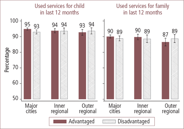
Notes: Sample sizes for "used services for study child in last year": Major cities advantaged (n = 3,529); major cities disadvantaged (n = 1,524); inner regional advantaged (n = 1,136); inner regional disadvantaged (n = 654); outer regional advantaged (n = 739); outer regional disadvantaged (n = 605). Sample sizes were slightly smaller for "used for family in last 12 months". For services used for the child, differences for remoteness × disadvantage, localities overall and disadvantage overall were not statistically significant, but differences for disadvantage within major cities were significant (p < .05). No significant differences were apparent for services used for the family.
Source: LSAC Wave 1, B and K cohorts combined
There was no evidence of differences in use of services for the family between the three geographic localities as defined by remoteness or between areas defined as disadvantaged and advantaged based on the area level unemployment rate.
Parents were also asked whether they had an unmet demand for services for their child or their family in the previous year. Figure 22 shows that the unmet need for such services was reported by a relatively small proportion of the parents. Around one in ten parents reported an unmet need for a service for their child in the last year. In outer regional areas, the unmet need was higher for disadvantaged rather than advantaged areas. This was the only significant variation on this measure. With regard to need for services for the family, there were no consistent differences between geographic localities or disadvantaged and advantaged areas.
Figure 22: Unmet need for services for the study child and for the family in the last 12 months in Australian advantaged and disadvantaged areas, by geographic locality
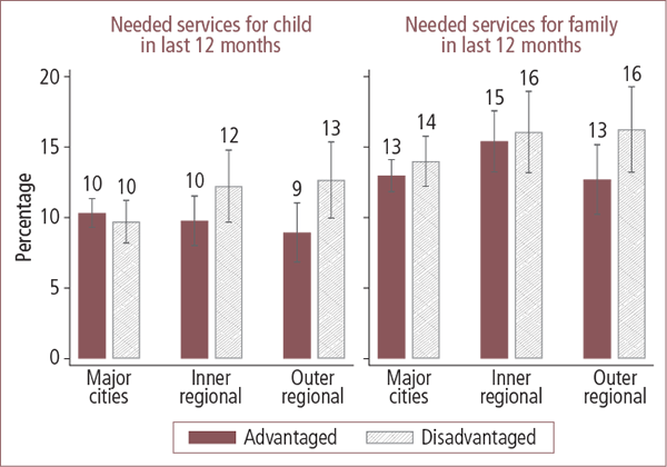
Notes: Sample sizes for "need services for study child in last year": Major cities advantaged (n = 3,404); major cities disadvantaged (n = 1,485); inner regional advantaged (n = 1,101); inner regional disadvantaged (n = 634); outer regional advantaged (n = 718); outer regional disadvantaged (n = 585). Sample sizes were slightly smaller for "need for family in last 12 months". For unmet need for services for child, differences by disadvantage were only significant for outer regional areas. For unmet need for services for family, differences for remoteness × disadvantage and localities overall were significant (p < .05), but differences by disadvantage overall and within localities were not significant. The tests of statistical significance are based on chi-square tests, not the confidence interval of the percentage as shown in the figure. Chi-square tests are more efficient than the confidence intervals and therefore, in this particular instance, there is not concordance in the statistical significance of these two methods of testing statistical significance.
Source: LSAC Wave 1, B and K cohorts combined
7.3 Summary
Overall, this section presents quite mixed findings with regard to how the social contexts of children vary by the remoteness and disadvantage of the area in which they live. While no differences between major city areas and inner and outer regional areas were apparent in relation to having regular contact with family, friends or neighbours, and having unmet needs for support, in terms of other indicators of social capital, there were some locality differences. Reporting to have received no help or not enough help from family and friends was most likely in the major cities - especially in advantaged areas - followed by inner regional and outer regional areas. Parents were involved in community groups or organisations at higher rates in the advantaged compared to disadvantaged areas; and in the regional areas more so than in the major cities. Also, low levels of neighbourhood belonging were less apparent in the regional compared to major city areas, especially outer regional areas, although in all localities a higher proportion of parents reported low levels of neighbourhood belonging in disadvantaged rather than advantaged areas.
Across the six socio-geographic areas in this analysis, service use for the study child and families was at fairly high levels and the level of unmet demand for services was low. Nevertheless, there were significantly lower rates of service use for study children living in disadvantaged areas in major cities compared to advantaged areas in major cities.
8. Children's educational activities
In this section, we examine children's educational environment. We begin with the home, focusing on the presence of children's books, and parents' reports of reading to their child. Television viewing is also a focus, as it has the potential to influence children's education through displacement of other more educational activities. We then look at attendance at child care and school, as well as extracurricular activities undertaken by children. In this section, unlike the others, we have explored differences by ages of children as well as socio-geographic area, as parents' attention to cognitive or learning development may apply more at certain ages, and child care and school settings vary considerably as children grow older.
The measures explored here are described in Table 8.
| Measure | Values | Notes |
|---|---|---|
| Books in the home | 30 or more books in the home (compared to fewer than 30 books, not shown) | Derived from question about how many children's books in the home. Parents are instructed to include library books. This was not available for 8-9 year olds. |
| Reading to children | Parents read to child daily | Available for children aged 2-3 years to 8-9 years. Response categories changed for 6-7 and 8-9 year old children such that "daily" includes the frequency 6-7 days per week. |
| Television watching | Child watches an average of 3 or more hours of TV per day on a weekday or weekend day | Based on parents' reports of the time the child spends watching television, on weekdays and weekend days. Not applicable for the B cohort at Wave 1. |
| Child care and early education | For children aged 0-1 years and 2-3 years, indicators of whether children were in any formal or informal child care are presented For children aged 4-5 years, an indicator of whether children attended preschool or child care is presented For children aged 6-7 years and 8-9 years, an indicator of whether children attended outside-school-hours care is presented | |
| Extra-curricular activities | Indicators of whether child participates in outside-school activities | Presented for children aged 6-7 and 8-9 years. Outside-school activities in the last 6 months for ages 6-7 are special or extra-cost activities in which the child participated that are not part of usual child care (e.g., swimming, music or movement classes). For 8-9 year olds, they are those in which the child regularly participates that are not part of usual outside-school-hours care. Parents were prompted with a list of possible activities. |
8.1 Educational activities in the home
Early exposure to learning in the home can come through the provision of learning materials and exposure to cognitively stimulating activities, such as reading to children. These types of activities have been associated with larger vocabularies and faster vocabulary growth, better listening comprehension, and better understanding of print concepts during early childhood (Huttenlocher, Haight, Bryk, Seltzer, & Lyons, 1991; Senechal, LeFevre, Hudson, & Lawson, 1996). In the large UK Effective Provision of Pre-School Education (EPPE) study, higher levels of parental involvement have also been related to children showing more independence, social competence, less antisocial behaviour and fewer worries (Sylva, Melhuish, Sammons, Siraj-Blatchford, & Taggart, 2004).
Number of children's books in the home
For the LSAC children, an indicator of access to educational resources is the number of children's books in the home. Figure 23 shows the proportion of children (aged 2-3 years, 4-5 years and 6-7 years) who lived in homes with 30 or more children's books (including library books). The clearest finding, apparent at all ages, is that children are less likely to have 30 or more books in the home in disadvantaged major city areas when compared to advantaged major city areas.
Figure 23: Children with 30 or more children's books in the home in Australian advantaged and disadvantaged areas, by geographic locality, aged 2-3 to 6-7 years
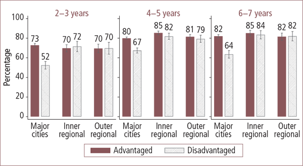
Notes: Sample sizes: Major cities advantaged (2-3 years: n = 2,099; 4-5 years: n = 4,368; 6-7 years: n = 2,011); major cities disadvantaged (n = 649; 1,229; 598); inner regional advantaged (n = 614; 1,354; 569); inner regional disadvantaged (n = 291; 571; 299); outer regional advantaged (n = 427; 1039; 430); outer regional disadvantaged (n = 229; 467; 246). Differences were significant (p < .05) for 4-5 and 6-7 year olds for localities overall, and for all age groups for remoteness × disadvantage, disadvantage overall, and disadvantage within major cities.
Source: LSAC Waves 1 to 2, K cohort; Waves 2 to 3, B cohort
Reading to children
Numerous studies report that parents reading regularly to preschoolers is related to better literacy when starting school (Bus, Vanijzendoorn, & Pellegrini, 1995; Raikes et al., 2006). Figure 24 shows the percentage of LSAC children to whom a parent reads on a daily basis (for 6-7 year olds, "daily" included the frequency of 6-7 days per week.). Percentages are presented separately for each age group because, as can be seen, the age at which this is a relatively common activity declines as children grow older and start reading for themselves. The percentage of children who were read to by a parent daily decreased steadily as children grew from 2-3 years to 6-7 years, and then decreased markedly at age 8-9 years. At age 8-9 years of age, fewer than 15% of children were read to by parents on a daily basis. (Given that reading to children at age 8-9 years of age is not normative, at this age reading to children may be indicative of learning difficulties).
Figure 24: Children read to by a parent daily in Australian advantaged and disadvantaged areas, by geographic locality, aged 2-3 to 8-9 years
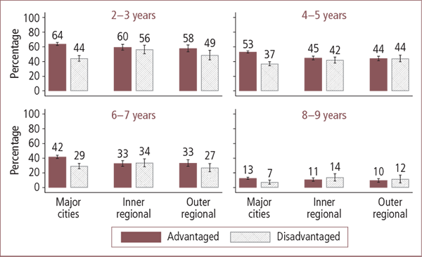
Notes: Sample sizes: Major cities advantaged (2-3 years: n = 2,099; 4-5 years: n = 4,368; 6-7 years: n = 2011; 8-9 years: n = 2,218); major cities disadvantaged (n = 649; 1,229; 598; 357); inner regional advantaged (n = 614; 1,354; 569; 700); inner regional disadvantaged (n = 291; 571; 299; 196); outer regional advantaged (n = 427; 1,039; 430; 561); outer regional disadvantaged (n = 229; 467; 246; 141). Differences were significant for all age groups for remoteness × disadvantage, for 4-5 and 6-7 year olds for localities overall, for all ages except 8-9 year olds for disadvantage overall, and for all ages for disadvantage within major cities.
Source: LSAC Waves 1 to 3, K cohort; Waves 2 to 3, B cohort
As with number of books in the home, associations between parents reading to their children and locality or disadvantage varied according to the ages of the children, with differences being at their greatest at 2-3 years of age. Overall, a significantly lower percentage of 2-3 year old children living in disadvantaged areas were read to daily when compared to those in advantaged areas, particularly within major cities. These differences were also apparent at other ages (although they were not statistically significant, overall, for 8-9 year olds).
Rates of parents reading daily to children varied by geographic locality for 4-5 year old and 6-7 year old children, with higher rates found for children living in major cities than in the inner or outer regional areas.
Television watching
High levels of television watching have been associated with lower learning outcomes, higher rates of behavioural and emotional problems (Anderson, Huston, Schmitt, Linebarger, & Wright, 2001; Fiorini, 2010; Smart et al., 2008) and increased likelihood of being overweight (Weicha et al., 2006). Possible reasons for the positive association between being overweight or obese and amount of television watching include reduced levels of physical activity, the influence of food advertising, and eating while viewing, all of which lead to greater calorie intake and lower energy expenditure (Jordan & Robinson, 2008). However, there are also other factors involved that explain the degree to which watching television can affect outcomes for children. In particular, the content of the programs watched has been found to be important, as well as the degree to which children passively watch, or are more actively engaged either with the program or with other people who are nearby. However, information about the content of television programs is not collected in LSAC.
For these analyses, we examined the percentage of children who usually watched three or more hours of television per day, as reported by parents. This cut-off of three hours has been used previously as an indicator of excessive time spent watching television (Smart et al., 2008).
Figure 25 shows the percentage of 2-3, 4-5, 6-7 and 8-9 year old children who usually watch three or more hours of television on a weekday or weekend day, by geographic locality and disadvantage. The greatest differences are evident according to the disadvantage of the area, with children living in disadvantaged areas being more likely to watch this amount of television than those living in advantaged areas. Within major cities, there were statistically significant differences between disadvantaged and advantaged areas, and this was apparent for all the age groups studied.
Figure 25: Children who watched three hours or more of television on a weekday or weekend day in Australian advantaged and disadvantaged areas, by geographic locality, aged 2-3 to 8-9 years
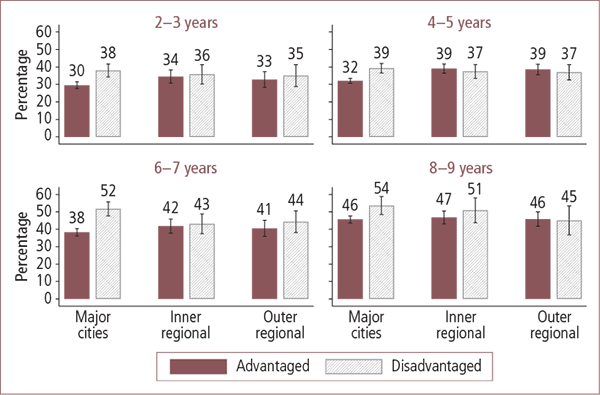
Notes: Sample sizes: Major cities advantaged (2-3 year olds: n = 2,099; 4-5 year olds: n = 4,368; 6-7 year olds: n = 2,011; 8-9 year olds: n = 2,218); major cities disadvantaged (n = 649; 1,229; 598; 357); inner regional advantaged (n = 614; 1,353; 569; 700); inner regional disadvantaged (n = 291; 571; 299; 196); outer regional advantaged (n = 427; 1,039; 430; 561); outer regional disadvantaged (n = 229; 468; 246; 141). Differences in percentages were significant for remoteness × disadvantage for all ages except 8-9 year olds, localities overall for 4-5 year olds only, disadvantage overall for all ages, and disadvantage within major cities for all age groups.
Source: LSAC Waves 2 to 3, B cohort; Waves 1 to 3, K cohort
8.2 Child care and early education
The availability of child care and preschool allows parents to go to work and can also provide children with learning and development opportunities to enhance their development. For instance, the UK EPPE project found that children who attended preschool had better cognitive and social and behavioural outcomes than those who did not (Sylva et al., 2004). Similar findings have been obtained by other studies (Beasley, 2002; Magnuson, Meyers, Ruhm, & Waldfogel, 2004). Australian research has also shown that formal child care has small associations with child wellbeing, some positive and some negative (e.g., Harrison, 2008; Leigh & Yamauchi, 2009).
Children aged 0-1 and 2-3 years old
Figure 26 shows the percentage of children aged 0-1 and 2-3 years in formal and informal child care by the six socio-geographic areas under analysis. Formal care includes day care centres, family day care and occasional care. Informal care includes being cared for by a grandparent, other relatives, parent living elsewhere, nanny or other person. Children may be in both formal and informal child care, or be in no child care at all. For formal child care rates, there was no variation among 0-1 year olds according to locality or disadvantage. Among 2-3 year old children, there was some variation overall, as well as specifically between geographic localities and between disadvantaged and advantaged areas. This figure shows that in major cities, participation in formal child care at 2-3 years of age was greater in advantaged areas, while in inner regional areas, disadvantaged areas had higher formal child care participation rates. For informal child care, there was no geographic variation for 0-1 year olds, but for 2-3 year olds there was significant variation by socio-demographic area. This was evident in outer regional areas, with significantly higher rates of informal care for 2-3 year olds in disadvantaged rather then advantaged areas.
Figure 26: Children in formal and informal child care in Australian advantaged and disadvantaged areas, by geographic locality, aged 0-1 and 2-3 years
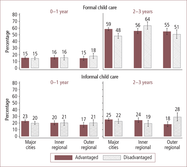
Notes: Sample sizes: Major cities advantaged (0-1 years: n = 2,084; 2-3 years: n = 2,099); major cities disadvantaged (n = 1,006; 649); inner regional advantaged (n = 672; 614); inner regional disadvantaged (n = 387; 291); outer regional advantaged (n = 435; 427); outer regional disadvantaged (n = 348; 229). For 0-1 year olds, differences in rates of formal and informal care were not significant for remoteness × disadvantage, localities overall or disadvantage overall. For 2-3 year olds, formal and informal care rates differed for remoteness × disadvantage. For this age group, formal care rates also varied for disadvantage overall, and by disadvantage in major cities and inner regional areas. Also, for this age group, informal care rates varied by disadvantage for outer regional areas, but there were no differences for locality overall or disadvantage overall.
Source: LSAC Waves 1 and 2, B cohort
Children aged 4-5 years old
At age 4-5 years, children may be in child care, preschool or even school. Very few children at this age are not in one of these arrangements (Harrison & Ungerer, 2005). Attendance at preschool, school or child care is variable across Australia, as the eligible age at which children can attend school varies between jurisdictions (Edwards, Taylor & Fiorini, 2011). The National Partnership Agreement on Early Childhood Education by the Council of Australian Governments on 29 November 2008 committed all State and Territory Governments to provide every child with access to a preschool program in the 12 months prior to full-time schooling.
Figure 27 shows the attendance of children aged 4-5 years at child care or preschools across geographic localities, excluding those children already in school. Very high rates of child care/preschool attendance are apparent in all localities. Some variation by locality and advantage is apparent, with the highest attendance rates being in advantaged areas of major cities and the lowest being in advantaged areas of outer regional areas. In major cities, the difference in participation rates between advantaged and disadvantaged regions was statistically significant, albeit small.
Figure 27: Children in child care or preschool in Australian advantaged and disadvantaged areas, by geographic locality, aged 4-5 years
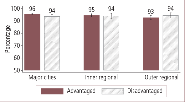
Notes: Sample sizes: Major cities advantaged (n = 4,368); major cities disadvantaged (n = 1,229); inner regional advantaged (n = 1,354); inner regional disadvantaged (n = 571); outer regional advantaged (n = 1,039); outer regional disadvantaged (n = 468). Percentages in child care/preschool varied for remoteness × disadvantage, localities overall, and by disadvantage for major city areas. Other differences were not statistically significant (p > .05). Excludes children already attending school.
Source: LSAC Wave 1, K cohort; Wave 3, B cohort
8.3 Outside-school activities
Findings from the Iowa Youth and Families Project suggested that active involvement of youth in church, sports, social clubs and leadership programs at school were associated with better grades, higher levels of social competence and lower levels of antisocial behaviour (Elder & Conger, 2000). Other studies of non-rural samples of children have also suggest that involvement in activities outside of school hours can be protective (Howie, Lukacs, Pastor, Reuben & Mendola, 2010).
One example of an outside-school activity is attendance at before- or after-school-hours care. Figure 28 shows quite low rates of attendance at outside-school-hours care across geographic localities, for both 6-7 year olds and 8-9 year olds. The highest participation rates are in advantaged major city areas, being significantly higher than the rates for disadvantaged areas in major cities. Overall, participation rates were higher in advantaged compared to disadvantaged areas, and variation by geographic locality was apparent, with higher proportions of children attending outside-school-hours care in major cities. This is consistent with other Australian research (Cassells & Miranti, 2012).
Figure 28: School-aged children's attendance at outside-school-hours care in Australian advantaged and disadvantaged areas, by geographic locality, aged 6-7 and 8-9 years
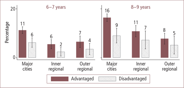
Notes: Sample sizes: Major cities advantaged (6-7 years: n = 2,011; 8-9 years: n = 2,218); major cities disadvantaged (n = 598; 357); inner regional advantaged (n = 569; 700); inner regional disadvantaged (n = 299; 196); outer regional advantaged (n = 430; 561); outer regional disadvantaged (n = 246; 142). Differences in outside-school-hours care rates were significant for remoteness × disadvantage, localities overall, disadvantage overall, by disadvantage in major city areas for both age groups, and by disadvantage in inner regional areas for 6-7 year olds.
Source: LSAC Waves 2 and 3, K cohort
Questions about children's involvement in other outside-school activities were included in Waves 2 and 3 of LSAC. Outside-school activities for 6-7 year olds were special or extra-cost activities in which the child participated in the last 6 months that were not part of the usual child care program (e.g., swimming, music or movement classes). For 8-9 year olds, outside-school activities were those in which the child regularly participated that were not part of the usual outside-school-hours care program (parents were prompted with a list of possible activities). Figure 29 shows the percentage of children aged 6-7 or 8-9 years who were involved in at least one outside-school activity. There was a difference between disadvantaged and advantaged areas, with higher participation rates in the latter. This difference was particularly marked in major cities.
Figure 29: School-aged children's attendance in outside-school activities in Australian advantaged and disadvantaged areas, by geographic locality, aged 6-7 and 8-9 years
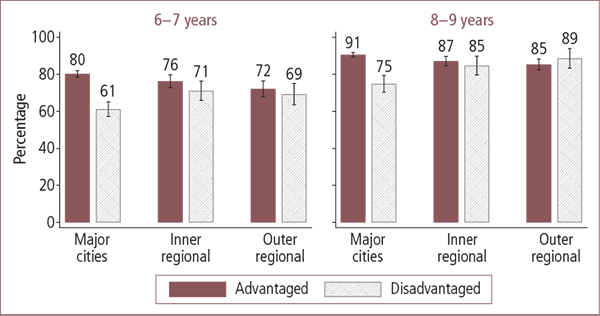
Notes: Sample sizes: Major cities advantaged (6-7 years: n = 2,011; 8-9 years: n = 2,218); major cities disadvantaged (n = 598; 357); inner regional advantaged (n = 569; 700); inner regional disadvantaged (n = 299; 196); outer regional advantaged (n = 430; 561); outer regional disadvantaged (n = 246; 141). Differences in rates were significant for remoteness × disadvantage, disadvantage overall, and by disadvantage in major cities for both age groups, and in inner regional areas for 6-7 year olds. Overall differences between localities were also apparent for 6-7 year olds.
Source: LSAC Waves 2 and 3, K cohort
8.4 Summary
As with previous sections of this report, the findings with regard to differences in children's educational contexts across socio-geographic areas are mixed. However, some differences are apparent, which are likely to reflect differences in parents' own levels of educational attainment and parents' engagement in the paid labour market (differences that were evident in Section 5 of this report). Also, Baxter et al. (2011) showed that parents' aspirations for their children's educational achievement varied considerably across the geographic localities of Australia (defined only based on remoteness), with parents in major cities being more likely than those in regional areas to expect children to reach university-level education. These aspirations are likely to be related to the investment that parents make in their young children's education.
On most of the educational measures, differences according to the disadvantage of the area were greater than differences between geographic localities. In particular, within major city areas, there were often significant differences between advantaged and disadvantaged areas. For example, there was some indication of lower levels of educational investment by parents in disadvantaged major city areas, with a smaller proportion of households having 30 or more children's books and fewer parents reading to their children daily. Children living in disadvantaged areas also watched more television compared to those living in advantaged areas, particularly in major city areas. Also, looking at school-aged children, those in disadvantaged areas of major cities were less likely to be enrolled in outside-school-hours care, or to participate in other outside-school activities. Some of these differences between disadvantaged and advantaged areas were evident outside of major cities, although to a lesser extent.
Differences across the socio-geographic areas in children's attendance at child care or preschool were evident, but such differences may reflect different parental needs for child care (for example, related to their employment arrangements), as well as different options available for care in their local environment. To determine to what extent the different child care or early education options might matter to children's outcomes, more detailed analyses of the characteristics of these arrangements would need to be explored. Similarly, it is apparent that participation in outside-school activities varies between socio-geographic areas, and Baxter et al. (2011) showed that the types of activities undertaken also vary by geographic locality. We return to examine whether differences such as these matter to children's outcomes in Section 9.
9. Child outcomes
This section now turns to the question of whether children in regional or rural areas experience a "tyranny of distance" or a "tyranny of disadvantage". Does distance from major cities explain the gaps in children's development in the regional or rural areas compared to children living in the major cities, or is it because many of these regional areas are disadvantaged compared to the cities? To answer this question, we tested whether there are differences in child outcomes by locality or disadvantage. Initially, we present descriptive information for the key child outcomes variables and then present multivariate analyses that take account of many of the different characteristics of children and families that have been described in earlier chapters.
9.1 Measures and methods
Children's outcomes are assessed in terms of cognitive outcomes, social-emotional outcomes and physical outcomes. The variables used here are described in Table 9. Throughout this section of the report, these measures are first analysed descriptively, and then using multivariate techniques. As noted in Table 9, the source of these data varies depending upon the measure analysed. However, for all measures, children are aged at least 4-5 years old, Therefore, information on children's outcomes from the B cohort at Waves 1 and 2 was not included.
| Domain | Outcome measure | Values | Notes |
|---|---|---|---|
| Cognitive | Receptive vocabulary | Scaled score Higher score = better outcome | Measured by the Peabody Picture Vocabulary Test (PPVT) Available for the B cohort at Wave 3 and the K cohort at all three waves (Dunn & Dunn 1997) |
| Non-verbal intelligence | Standardised score Higher score = better outcome | Measured by the Matrix Reasoning test Available for the K cohort at Waves 2 and 3 only | |
| Social-emotional | Emotional and behavioural problems in the abnormal range | 0 (not in abnormal range: Strengths and Difficulties Questionnaire [SDQ] total difficulties score of 0-16) 1 (score in abnormal range: SDQ total difficulties score of 17-35) | Total Problem Score from the SDQ (sum of parent-report scores on hyperactivity, emotional problems, peer problems, and conduct problems sub-scales) Available for the B cohort at Wave 3 and the K cohort at all three waves. (Goodman, 1997) |
| Physical | Overweight (relative to normal or underweight) | 0 (not overweight) 1 (overweight) | Score derived from child weight status, based on BMI Available for the B cohort at Wave 3 and the K cohort at all three waves |
To undertake multivariate analyses of these outcomes, a range of the variables highlighted in this report are used. Some have been used to examine each outcome variable, but others have been selected specifically for certain outcomes, as informed by the existing literature on predictors of children's outcomes. A summary of the measures used in the multivariate analyses is given in Table 10.
| Variable | Measure | Value (reference) | Cognitive | Social- emotional | Physical |
|---|---|---|---|---|---|
| Socio-geographic area | Remoteness × disadvantage | X | X | X | |
| Child/survey control variables | Child gender | Boy (ref. = girl) | X | X | X |
| Indigenous child | Indigenous child (ref. = not Indigenous) | X | X | X | |
| Cohort/wave | Controls for cohort and wave | X | X | X | |
| Demographics | Family form | Single parent (ref. = couple or other family forms) | X | X | X |
| Mothers' country of birth and English-language proficiency | Mother born overseas, only English or good English-language proficiency; mother born overseas, poor English language (ref. = mother born in Australia) a | X | X | X | |
| Parental education | Either parent (or single parent) has a bachelor degree or higher (ref. = neither parent has bachelor degree or higher) | X | X | X | |
| Family joblessness | Jobless family (ref. = at least one parent is employed) | X | X | X | |
| Financial hardships | Number of financial hardships (0, 1, 2, 3+) | X | X | X | |
| Housing tenure | Own or buying house (ref. = renting or other housing) | X | X | X | |
| Neighbourhood and social contexts | English-speaking in area | Percentage English-speaking in local area | X | X | X |
| Safe neighbourhood | Does not agree neighbourhood is safe (ref. = agrees neighbourhood is safe) | X | X | X | |
| Good parks b | Does not agree neighbourhood has good parks, playgrounds and play spaces (ref. = agrees neighbourhood has good parks, playgrounds and play spaces) | X | |||
| Unmet demand for support | Has unmet demand for support or help (ref. = no unmet demand for support or help) | X | X | X | |
| Involvement in volunteer or community groups | Involved in volunteer groups (ref. = not involved in volunteer groups) | X | X | X | |
| Neighbourhood belonging | Lower neighbourhood belonging (ref. = not lower neighbourhood belonging) | X | X | X | |
| Services use | Child used services in previous 12 months (ref. = child did not use services in previous 12 months) | X | X | X | |
| Parent wellbeing and parenting | Parent mental health | Either parent has serious mental health risk (ref. = neither parent has serious mental health risk) | X | X | X |
| Alcohol consumption | Either mother or father binge drinker; either mother or father abstains from alcohol | X | X | X | |
| Parental weight c | Either parent is overweight (ref. = neither parent is overweight) | X | |||
| Parenting: Warm parenting | Either parent lower parental warmth (ref. = neither parent lower parental warmth) | X | X | X | |
| Parenting: Angry parenting | Either parent higher angry parenting (ref. = neither parent higher angry parenting) | X | X | X | |
| Books in the home d | 30 or more books in the home (ref. = fewer than 30 books) | X | |||
| High TV watching | Watches 3 hours or more TV per day (ref. = watches less than 3 hours TV) | X | X | X |
Notes: a For multivariate analyses, missing mothers' details are replaced with fathers' characteristics (e.g., in single-father family). b While opportunities for play is an important factor for child overweight (Harrison et al., 2011), it has not been found to be the case for other outcomes (e.g., Edwards & Bromfield, 2009). c There is no evidence that children's cognitive development or social-emotional wellbeing is affected by having a parent overweight, particularly given that many other family functioning measures were included in the statistical models. d Having books has been associated with a number of cognitive outcomes (Huttenlocher et al., 1991; Senechal et al., 1996) but is less relevant to social-emotional wellbeing and overweight, particularly given that parenting style was included in the statistical models. For 8-9 year olds, number of books in the home was set to be equal to the number of books in the home when these children were aged 6-7 years, since this information was not collected for 8-9 year olds.
Note that some of the variables examined in earlier sections of the report were not included in the multivariate analyses. Some were excluded because they were only available at selected waves. Others were excluded because they varied considerably across waves, either in the way they were collected (e.g., the child care variables), or in their meaning (e.g., reading to children by parents of 8-9 year olds is not normative by this age and is quite likely to reflect those children having learning difficulties).
Random effects multivariate regression models were used to find out whether any of these factors explain locational differences. To obtain the most precise estimates, data were pooled from each cohort and wave, taking account of cohort and wave differences in the models using dummy variables. While the clustering that occurs due to having multiple measures of the same child outcomes are accounted for directly by a random effects multivariate regression model, where possible we use robust standard errors to account for clustering that occurs by virtue of the fact that many children live in the same geographic area.10
The coefficients in these models represent the amount of change in the dependent variable associated with the presence of a particular characteristic, but because they are derived from multiple records per person, they represent both differences across groups of children (at any one wave) and differences across waves for individual children. Some characteristics do not change at all across waves (such as sex of the child), while some do have the potential to change (e.g., parenting style or mental health). For those variables that may change across waves, the estimated coefficient will reflect these changes across the waves, as well as between groups of children. The coefficients cannot be used to draw conclusions about causal relationships. They instead are used to describe associations between variables.
For the continuous measures (the two cognitive outcomes), random effects ordinary least squares was used, with results presented as coefficients. The coefficients are easily interpreted as the difference in an outcome measure associated with having that characteristic.
For those outcomes coded as binary variables (the social-emotional and physical outcomes), random effects logistic regression was used, with results presented as odds ratios. For binary variables, the "odds" of having a particular outcome is the probability of having it as a ratio of the probability of not having it. Odds ratios are an estimate of how the "odds" vary for those with and without a particular characteristic. They provide an indication of whether this outcome (e.g., being overweight) is more likely (if the odds ratio is greater than 1) or less likely (if the odds ratio is less than 1) for those with a particular characteristic, relative to not having this characteristic.
For each outcome measure, four models were estimated:
- Model 1 included only cohort and wave control variables. Two indicators for geographic locality were included - inner regional and outer regional areas - with major cities being the reference category. An indicator for disadvantaged areas was included, with the reference category being advantaged areas. To test whether the effect of disadvantage was stronger or weaker in inner or outer regional areas, compared to major cities, two interaction terms were included - inner regional by disadvantage and outer regional by disadvantage. Using this approach, it was possible to test (a) whether there were differences in children's outcomes according to geographic locality; (b) whether children's outcomes differed when living in a disadvantaged area; and (c) whether living in a disadvantaged area had stronger or weaker associations with children's outcomes in the different geographic localities.
- In Model 2, child and family demographic variables were added.
- Model 3 included all of the above as well as neighbourhood and social contextual variables.
- In Model 4, in addition to the variables in Model 3, the most proximal factors were included, namely parenting and parent wellbeing variables.
Table 11 and subsequent tables of results show just the results for the socio-geographic variables. For the continuous measures (the two cognitive outcomes), in addition to the estimated coefficients, model statistics have been given: the size of the sample included in the analyses, the number of children this relates to, and the overall R-squared value. The R-squared value gives an estimate of the amount of overall variance explained by the model. For each outcome measure, comparisons between the models are provided, showing the significance of the change in the R-squared value as further characteristics are added.
For the binary outcome variables, the log-likelihood statistic is presented instead of the overall R-squared value, which is a measure of the goodness of fit of the model.
All multivariate results are presented in Appendix B. Table B1 presents the final model for each outcome, and subsequent tables present each of the models one outcome at a time. The model statistics presented in Table B1 includes the intraclass correlation coefficient (?), which is equal to the proportion of total variance contributed by the child-level variance. The intraclass correlation coefficient is an indication of the importance of taking into account the fact that multiple records from individual children are included in the analyses.
A number of the variables listed in Table 10 are subject to item non-response. To maximise the sample available for analyses, variables that were subject to some non-response were re-coded, such that respondents with missing data on that item could be included. Each variable was initially coded to 0 or 1, with 0 indicating the absence of some characteristics and 1 indicating the presence of that characteristic. This indicator was missing for those without this information provided. For example, having higher angry parenting was equal to 0 for those whose angry parenting was not in the upper range, was equal to 1 if in the upper range, and otherwise was missing. To include those with missing data on this item, an indicator of having missing higher angry parenting data was included as if it was another category to this item. This still allows the comparison of those with genuine values of 0 and 1. This was done for the following variables: unmet demand for support or help, involvement in volunteer groups, low neighbourhood belonging, child using services in previous 12 months, parent having a serious mental health risk, parental alcohol use, and parent having higher angry parenting or lower warm parenting.
9.2 Cognitive outcomes
Cognitive outcomes were assessed using two different measures. Receptive vocabulary, assessed with the Peabody Picture Vocabulary Test (PPVT), was measured at ages 4-5 years, 6-7 years and 8-9 years (Figure 30). Non-verbal intelligence, assessed with the Matrix Reasoning test, was measured at 6-7 years and 8-9 years (Figure 31).
Receptive vocabulary
Figure 30 shows that, overall, receptive vocabulary increases as children age, with substantial increases occurring between 4-5 to 6-7 years and between 6-7 to 8-9 years. Overall, children living in disadvantaged areas had lower levels of receptive vocabulary than children living in advantaged areas across the three age groups. There were not consistent differences across locations for the three age groups, although it does appear that the difference in receptive vocabulary between advantaged and disadvantaged areas was greater in major cities than in the regional areas.
Figure 30: PPVT scores in Australian advantaged and disadvantaged areas, by geographic locality, aged 4-5 to 8-9 years
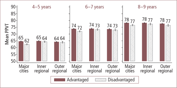
Notes: Sample sizes: Major cities advantaged (4-5 years: n = 4,050; 6-7 years: n = 1,966; 8-9 years: n = 2,200); major cities disadvantaged (n = 1,123; 576; 355); inner regional advantaged (n = 1,258; 545; 691); inner regional disadvantaged (n = 533; 292; 195); outer regional advantaged (n = 987; 407; 550); outer regional disadvantaged (n = 413; 233; 140). Differences for remoteness × disadvantage and disadvantage overall were statistically significant (p < .05). Differences for localities overall were only significant for 8-9 year olds. Differences by disadvantage within localities were not significant for inner regional areas for 6-7 and 8-9 year olds, and outer regional areas for 4-5 and 6-7 year olds.
Source: LSAC Wave 3, B cohort; Waves 1 to 3, K cohort
At age 4-5 years, children living in disadvantaged areas in major cities had significantly lower levels of receptive vocabulary than any of the other five groups. There were no statistically significant differences between children living in advantaged major city areas and those in inner and outer regional areas (either advantaged or disadvantaged).
When children were two years older, at 6-7 years of age, those living in disadvantaged areas of major cities had significantly lower receptive vocabulary than those living in advantaged major city areas, advantaged outer regional areas and advantaged inner regional areas. There were no other statistically significant differences.
At age 8-9 years, children living in disadvantaged major city areas had significantly lower receptive vocabulary than children living in advantaged major city areas. Children living in disadvantaged outer regional areas also had significantly lower levels of receptive vocabulary than those living in advantaged outer regional areas. It is important to note that while the differences noted are statistically significant, they were quite small.
It is unclear, however, whether these differences between geographic locality and disadvantaged areas are due to systematic differences in the demographic characteristics of the child, their family characteristics, differences in neighbourhood and social contexts, and parenting and parent wellbeing. As discussed above, multivariate analyses were used to identify whether variation between socio-geographic areas was apparent after taking account of such differences in characteristics. Table 11 shows just the results for the socio-geographic variables for each of Models 1 through 4. See Appendix B for the full multivariate results.
| Model 1: Child/cohort/ wave controls | Model 2: Model 1 plus demographics | Model 3: Model 2 plus neighbourhood and social contexts | Model 4: Model 3 plus parenting and family | |
|---|---|---|---|---|
| Coefficients | ||||
| Geographic locality (ref. = major city) | ||||
| Inner regional | 0.01 | -0.02 | -0.34 * | -0.30 * |
| Outer regional | -0.56 *** | -0.48 ** | -0.81 *** | -0.74 *** |
| Disadvantaged | -0.85 *** | -0.34 * | -0.16 | -0.11 |
| Inner regional & disadvantaged (interaction) | 0.56 * | 0.18 | 0.05 | 0.02 |
| Outer regional & disadvantaged (interaction) | 0.97 *** | 0.62 * | 0.40 | 0.31 |
| Child/cohort/wave controls | X | X | X | X |
| Demographics | X | X | X | |
| Neighbourhood and social contexts | X | X | ||
| Parenting and family | X | |||
| Model statistics | ||||
| Number of observations | 16,416 | 16,416 | 16,416 | 16,416 |
| Number of children | 8,799 | 8,799 | 8,799 | 8,799 |
| Overall R-square | 0.53 | 0.57 | 0.57 | 0.58 |
| Test of difference from previous model (chi-square) | n. a. | *** | *** | *** |
Notes: See Table 9 for descriptions of outcome measures and Table 10 for details of the variables included in each model. * p < .05; ** p < .01; ***p < .001;
Source: LSAC Wave 3, B cohort; Waves 1 to 3, K cohort
In Model 1, the results suggest that, compared to children living in advantaged areas, children living in disadvantaged areas had significantly lower levels of receptive vocabulary. Also, compared to children living in major city areas, children living in outer regional areas had significantly lower levels of receptive vocabulary.11
The addition of child and family demographic characteristics meant that the interaction for inner regional areas was no longer statistically significant. The other differences were reduced in size but still statistically significant. Between Model 1 and 2, the size of the differences for living in a disadvantaged area reduced by 60%, suggesting that child and family characteristics partly explain differences between advantaged and disadvantaged areas.
Most of the child and family demographic characteristics had statistically significant associations with children's receptive vocabulary in the expected direction. Boys and children who were Aboriginal or Torres Strait Islanders had lower levels of receptive vocabulary, while children living in jobless households and those living in households experiencing financial hardship also had significantly lower levels of receptive vocabulary. Children living in households where their mother was born overseas, particularly those whose mothers had poor English, also had worse receptive vocabulary. Children living in households where at least one parent was university-educated or who were home-owners (outright or paying off a mortgage) had higher levels of receptive vocabulary. Children living in single-parent households did not have worse receptive vocabulary than children living in couple-parent households. (For more detailed information, see Appendix B.)
When neighbourhood and social contexts (Model 3) were included, the disadvantaged areas indicator and the interaction between disadvantaged areas and outer regional areas were reduced further and no longer statistically significant. Children living in outer regional areas still had significantly lower levels of receptive vocabulary compared to children living in major city areas, and children living in inner regional areas also had significantly lower levels of receptive vocabulary. A few neighbourhood and social context variables were significantly associated with children's receptive vocabulary at this step, and were the likely candidates for explaining differences in children's receptive vocabulary between disadvantaged and advantaged outer regional areas.
One relates to the language environment where families reside. Results from the modelling suggest that living in an area with a higher percentage of residents who speak English provides a richer environment for learning the language, as children residing in these areas had significantly higher levels of receptive (English) vocabulary. Given that advantaged areas had a higher percentage of English speakers, this may also explain some of the differences between disadvantaged and advantaged areas.
Also, children who had a mother who was involved in a volunteer or community group had higher levels of receptive vocabulary, and children who had a parent who reported lower levels of neighbourhood belonging had lower levels of receptive vocabulary. This suggests that for children living in disadvantaged areas, parental engagement with the community is an important protective factor. One of the mechanisms could be that parents who are more engaged in their community have children who are more engaged with school and outside-school activities, as was found in the Iowa Youth and Family Project (Elder & Conger, 2000). Given that this information was only collected at age 8-9 years, we did not include engagement in outside-school activities in the statistical models, but it may be that these more engaged parents are able to create social opportunities for their children that benefit their receptive vocabulary.
Model 4 takes account of differences in parenting and family functioning. After the addition of these variables, children living in major cities still had significantly higher levels of receptive vocabulary than children living in inner and outer regional areas. Several parenting and family functioning variables were significantly associated with children's receptive vocabulary. As would be expected, relatively high levels of angry parenting were associated with significantly lower levels of receptive vocabulary, as was watching three or more hours of TV a day. Having 30 or more children's books in the home was associated with greater levels of children's receptive vocabulary. Children with at least one parent who was a binge drinker had lower levels of receptive vocabulary than children of parents who did not engage in binge drinking but still consumed some alcohol. On the other hand, children of parents where there was at least one parent who abstained from drinking alcohol altogether had even lower levels of receptive vocabulary compared to children of parents who drank alcohol responsibly. This particular finding warrants further explanation. Previous research suggests that abstainers have higher levels of depressive and anxiety symptoms than light or moderate drinkers (Alati et al., 2004; 2005; Power, Rodgers, & Hope, 1998; Rodgers et al., 2000), and abstainers have been found to have poorer social relationships than light or moderate drinkers (Lucas, Windsor, Caldwell, & Rodgers, 2010). Therefore poor mental health and lack of social integration may explain children's lower levels of receptive vocabulary in these family situations.
In summary, the results from the random effects regression models suggest that there were differences in children's receptive vocabulary between disadvantaged and advantaged areas as well as between major city areas and inner and outer regional areas, when not taking other variables into account. Family demographic characteristics (such as parental education), exposure to environments where English is spoken more frequently, and community involvement and a sense of belonging are likely factors that explain differences in children's level of receptive vocabulary between disadvantaged and advantaged areas. Most striking is the fact that the tyranny of distance from major city areas is so persistent. Differences in children's receptive vocabulary between major city and inner and outer regional areas were still evident even when the large number of socio-demographic, social context and family variables were included.
Non-verbal intelligence
As another measure of cognitive development, we now explore differences in children's non-verbal intelligence, here assessed by the Matrix Reasoning test. This test is not designed to measure change over time, as the test score is a relative measure or rank of where children sit compared to their peers. An examination of the mean Matrix Reasoning scores reported in Figure 31 for 6-7 and 8-9 year olds illustrate this point; there is no evidence of change with child age.
Figure 31: Children's Matrix Reasoning scores in Australian advantaged and disadvantaged areas, by geographic locality, aged 6-7 and 8-9 years
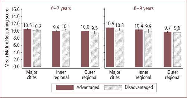
Notes: Sample sizes: Major cities advantaged (6-7 years: n = 1,995; 8-9 years: n = 2,198); major cities disadvantaged (n = 591; 354); inner regional advantaged (n = 563; 691); inner regional disadvantaged (n = 298; 195); outer regional advantaged (n = 422; 549); outer regional disadvantaged (n = 244; 141). Differences for remoteness × disadvantage, localities overall and disadvantage overall were all statistically significant (p < .05). Differences between disadvantaged and advantaged areas within localities were significant for both age groups in major cities and for 6-7 year olds in outer regional areas.
Source: LSAC Waves 2 and 3, K cohort
This figure shows that, overall, higher non-verbal intelligence scores were achieved by children in major cities, with the lowest average scores being for those in outer regional areas. This was true for both age groups examined. Also, differences between children living in advantaged and disadvantaged areas were consistently reported for both age groups, with higher average scores in the advantaged areas. As such, children living in advantaged major city areas had significantly higher non-verbal intelligence scores than children in disadvantaged major city areas for both age groups. Six- to seven-year-old children living in disadvantaged outer regional areas also had significantly lower scores than children living in advantaged outer regional areas.
The results from the random effects regression for Model 1 confirm the findings apparent in Figure 31. The results indicate that children living in major cities have significantly higher scores on Matrix Reasoning than children living in inner regional and outer regional areas (Table 12). Children living in disadvantaged areas also had significantly lower levels of non-verbal reasoning than those in advantaged areas. There was no evidence that the influence of disadvantaged areas was different between geographic localities (the interaction effects were not statistically significant).
| Model 1: Child/cohort/ wave controls | Model 2: Model 1 plus demographics | Model 3: Model 2 plus neighbourhood and social contexts | Model 4: Model 3 plus parenting and family | |
|---|---|---|---|---|
| Coefficients | ||||
| Geographic locality (ref. = major city) | ||||
| Inner regional | -0.59 *** | -0.39 *** | -0.45 *** | -0.44 *** |
| Outer regional | -0.87 *** | -0.56 *** | -0.61 *** | -0.61 *** |
| Disadvantaged | -0.24 * | -0.09 | -0.05 | -0.03 |
| Inner regional & disadvantaged (interaction) | 0.38 | 0.31 | 0.29 | 0.27 |
| Outer regional & disadvantaged (interaction) | 0.19 | 0.13 | 0.09 | 0.07 |
| Child/cohort/wave controls | X | X | X | X |
| Demographics | X | X | X | |
| Neighbourhood and social contexts | X | X | ||
| Parenting and family | X | |||
| Model statistics | ||||
| Number of observations | 8,189 | 8,189 | 8,189 | 8,189 |
| Number of children | 4,388 | 4,388 | 4,388 | 4,388 |
| Overall R-square | 0.02 | 0.05 | 0.06 | 0.06 |
| Test of difference from previous model (chi-square) | n. a. | *** | *** | *** |
Notes: See Table 9 for descriptions of outcome measures and Table 10 for details of the variables included in each model. * p < .05; ** p < .01; * **p < .001;
Source: LSAC Waves 2 and 3, K cohort
The child and family demographic variables that were introduced in Model 2 explain the gap between advantaged and disadvantaged areas in Matrix Reasoning scores, such that this difference was no longer statistically significant when these variables were added to the model. Children living in inner and outer regional areas still had significantly lower non-verbal reasoning than in major cities, although the gap had been partially bridged by the inclusion of child and family demographic variables.
The child and family demographic variables that had the strongest associations with non-verbal reasoning, hence explaining the bridging of the disadvantaged area gap, were:
- having a parent in the household with a university degree, which was associated with children having higher non-verbal reasoning scores; and
- being of Aboriginal or Torres Strait Islander, associated with children having significantly lower non-verbal reasoning scores compared to other children.
- Other significant, although smaller associations, were apparent for the level of financial hardship experienced by families (with higher levels of hardship associated with lower scores on non-verbal reasoning) and having parents who owned or who were paying off a mortgage, compared to renting (associated with children having higher non-verbal reasoning scores). After the inclusion of parenting and family variables in Model 4, both of these variables no longer had a significant association with non-verbal reasoning (see Appendix B for more details on the statistical significance of other variables).
Another key variable was whether the mother was born overseas and had poor English; compared to children whose mothers were not born overseas, children who had mothers born overseas and with poor English had significantly higher non-verbal reasoning. This result is in the opposite direction to that found for the measure of receptive vocabulary.
The gender of the child also was a significant variable - boys had significantly lower Matrix Reasoning scores than girls.
Neighbourhood and social contexts (Model 3) did not seem to explain any of the socio-geographic differences between children on Matrix Reasoning, with the coefficients on the socio-geographic indicators being unchanged from Model 2. Parent wellbeing and parenting also did not explain the differences across localities in Matrix Reasoning scores - the coefficients for the indicators of locality were virtually identical in Model 4 as in Model 3. Nonetheless, it is important to note a few neighbourhood and social context and parent wellbeing and parenting variables had significant associations with children's non-verbal reasoning; parental involvement in community or volunteer groups and having more than 30 books in the home were both associated with higher non-verbal reasoning scores.
In summary, the results from the random effects multivariate regression suggest that there is a tyranny of distance - differences between children living in major city areas and inner and outer regional areas - in children's non-verbal intelligence that cannot be explained by the rich set of variables in the model. In contrast, differences in non-verbal intelligence between children living in disadvantaged and advantaged major city areas seems to be largely accounted for by demographic differences between children and their families living in these two different areas.
9.3 Social-emotional outcomes
Child behavioural and emotional outcomes are measured using the Strengths and Difficulties Questionnaire (Goodman, 1997). These subscales include measures of:
- hyperactivity - fidgetiness, concentration span and impulsiveness;
- emotional symptoms - frequency of display of negative emotional states (e.g., nervousness, worry);
- peer problems - ability to form positive relationships with other children; and
- conduct problems - tendency to display problem behaviour when interacting with others.12
Each subscale is calculated from the mean score of five questions asked of the respondent. These subscales can be added together to form an SDQ total difficulties score that can be interpreted as an equally weighted measure of these four domains of behavioural problems. The SDQ also has cut-offs that suggest that children who score above these are at risk of being in the clinical range for behavioural or emotional problem. This was used in this report, such that children with a total difficulties score of 17-35, rather than lower than this, were said to have emotional or behavioural problems. LSAC contains both parent and teacher responses to the SDQ. We chose parent reports to minimise the amount of missing data.
Figure 32 shows the percentage of children at risk of emotional or behavioural problems by age, as derived from the SDQ total difficulties score. The rate of children experiencing emotional or behavioural problems does not appear to increase with age; in fact, there appear to be slightly lower rates of emotional or behavioural problems by 8-9 years of age compared to the other age groups.
Figure 32: Children with emotional or behavioural problems in Australian advantaged and disadvantaged areas, by geographic locality, aged 4-5 to 8-9 years
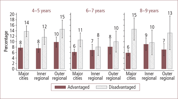
Notes: Sample sizes: Major cities advantaged (4-5 years: n = 4,066; 6-7 years: n = 1,960; 8-9 years: n = 1,949); major cities disadvantaged (n = 1,139; 573; 294); inner regional advantaged (n = 1,273; 557; 632); inner regional disadvantaged (n = 548; 286; 168); outer regional advantaged (n = 993; 422; 503); outer regional disadvantaged (n = 458; 238; 120). Differences for remoteness × disadvantage and disadvantage overall were all statistically significant (p < .05). Differences for localities overall were not significant for any age group. Differences for disadvantage within localities were not significant for inner and outer regional areas for 6-7 and 8-9 year olds.
Source: LSAC Wave 3, B cohort; Waves 1 to 3, K cohort
Chi-square tests suggest that children living in disadvantaged areas had significantly higher rates of emotional or behavioural problems than those living in advantaged areas and this was particularly apparent in major cities, but also was apparent for 4-5 year olds in inner regional areas. Overall, there were no significant differences in rates of emotional or behavioural problems between the three geographic localities.
The random effects logit models pool information from the three age groups so that there is a larger sample size for statistical estimation and hence more statistical precision to detect significant differences. Table 13 provides a summary of the models.
| Model 1: Child/cohort/ wave controls | Model 2: Model 1 plus demographics | Model 3: Model 2 plus neighbourhood and social contexts | Model 4: Model 3 plus parenting and family | |
|---|---|---|---|---|
| Odds ratios | ||||
| Geographic locality (ref. = major city) | ||||
| Inner regional | 1.19 | 0.99 | 1.03 | 1.10 |
| Outer regional | 1.39 | 1.12 | 1.22 | 1.35 |
| Disadvantaged | 2.16 *** | 1.54 ** | 1.49 ** | 1.51 ** |
| Inner regional & disadvantaged (interaction) | 0.63 | 0.81 | 0.81 | 0.82 |
| Outer regional & disadvantaged (interaction) | 0.73 | 0.84 | 0.85 | 0.76 |
| Child/cohort/wave controls | X | X | X | X |
| Demographics | X | X | X | |
| Neighbourhood and social contexts | X | X | ||
| Parenting and family | X | |||
| Model statistics | ||||
| Number of observations | 16,087 | 16,087 | 16,087 | 16,087 |
| Number of children | 8,470 | 8,470 | 8,470 | 8,470 |
| Log likelihood | -3902 | -3732 | -3680 | -3399 |
| Test of difference from previous model (chi-square) | n. a. | *** | *** | *** |
Notes: See Table 9 for descriptions of outcome measures and Table 10 for details of the variables included in each model. * p < .05; ** p < .01; * **p < .001.
Source: LSAC Wave 3, B cohort; Waves 1 to 3, K cohort
Results from Model 1 suggest that, compared to children living in advantaged areas, children living in disadvantaged areas were more likely to experience emotional or behavioural problems (odds ratio of 2.2). There were no significant differences in the rates of emotional or behavioural problems between major city, inner and outer regional areas. The non-significant interaction terms suggest that the influence of disadvantaged areas was similar across the three geographic localities.
When child and family demographic variables were included (Model 2), then the difference in the rates of emotional or behavioural problems of those children living in advantaged and disadvantaged areas was reduced somewhat (odds ratios declining from 2.2 to 1.5), but was still statistically significant. This suggests that differences in the socio-demographic composition of families explain some of the differences between disadvantaged and advantaged areas. Results for this model showed that children living in a jobless household, those living in families who experienced financial hardship, or those with mothers who were born overseas with poor English were more likely to experience emotional or behavioural problems.13 Children with at least one parent with a university education or with parents who owned or were buying their home were less likely to have emotional or behavioural problems. Boys and children who were Aboriginal or Torres Strait Islanders were more likely to have emotional or behavioural problems. (See the results for these variables in Model 4, presented in Appendix B, for more detail.)
The introduction of neighbourhood and social context variables (Model 3) and parenting and family variables (Model 4) did not change the influence of living in disadvantaged areas on children's likelihood of experiencing emotional or behavioural problems. Children living in disadvantaged areas were more likely to be at risk of emotional or behavioural problems than children living in advantaged areas (odds ratios of 1.5 in each model), even after taking into account differences in neighbourhood and social contexts, and parenting and family factors.
Nevertheless, readers may be interested in the statistically significant factors that were associated with a higher likelihood of children experiencing emotional or behavioural problems. The following were all associated with higher risks of emotional or behavioural problems:
- relatively high levels of angry parenting;
- at least one parent having a mental health problem;
- parents reporting their neighbourhood as unsafe;
- having lower neighbourhood belonging and unmet demand for support;
- parents not being involved in volunteer or community groups;
- either parent abstaining from alcohol;
- children having used services in the past 12 months; and
- high levels of TV watching.
Relatively high levels of parental irritability and anger towards the study child (angry parenting) was by far the strongest risk factor (with an odds ratio of 7.3), with the next strongest risk factor being parent mental health problems.
Several of these statistically significant variables were of note. First, that a higher level of service use for the child was associated with a higher likelihood of child emotional or behavioural problems. It is not clear why this was the case, but it could be that parents were accessing services to address this issue or it is possible that these children generally required more services. Second, having a parent who participated in a volunteer or community group was protective, with these children being at lower risk of emotional or behavioural problems. Third, compared to children who had parents who drank alcohol but did not binge drink, children who had parents who abstained from any drinking had a higher risk of emotional or behavioural problems. Given that abstention from alcohol is a proxy for higher levels of distress (Alati et al., 2004) and lack of social integration (Lucas et al., 2010), these factors are likely to underlie this result.
In general, the results from the statistical modelling suggest that unlike for cognitive outcomes, children living in disadvantaged areas had higher levels of emotional or behavioural problems. Family demographic variables explained part of this relationship, but the association with living in disadvantaged areas remained, even after the introduction of neighbourhood and social capital, and parent wellbeing and parenting variables. This suggests that while part of the explanation is that more disadvantaged families live in areas of higher unemployment, other factors that were not included in our models explain these differences.
9.4 Physical wellbeing outcomes
Childhood obesity has been increasing in Australia (Booth et al., 2003). The prevalence of being overweight or obese is very high; for example, data from the Australian National Children's Nutrition and Physical Activity Survey (2007) suggest that the prevalence of being overweight or obese in children aged 2-12 years was 22% (AIHW, 2009).
In LSAC, being overweight or obese is determined by using the child's height and weight to calculate BMI. The definition of overweight and obese used is taken from the International Obesity Task Force (Cole, Bellizzi, Flegal & Dietz, 2000), which takes account of the child's BMI for age and gender. Height was the average of two height measurements using stadiometers, and weight was measured using digital scales.
Figure 33 shows the percentage of children who were classified as overweight or obese (as opposed to underweight or normal weight) across geographic localities and disadvantaged and advantaged areas. For 4-5 year olds, children living in disadvantaged inner regional areas had higher rates of being overweight than those living in advantaged inner regional areas.14 There were no other statistically significant differences between regional areas or between disadvantaged and advantaged areas for this age group. Six to seven year old and 8-9 year old children living in advantaged major city areas had significantly lower rates of overweight than those living in disadvantaged major city areas. This gap was slightly bigger for the older age group.
Figure 33: Children who are classified as overweight or obese in Australian advantaged and disadvantaged areas, by geographic locality, aged 4-5 to 8-9 years
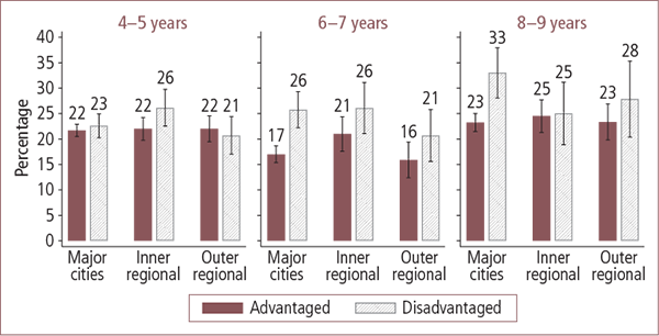
Notes: Sample sizes: Major cities advantaged (4-5 years: n = 4,326; 6-7 years: n = 1,996; 8-9 years: n = 2,204); major cities disadvantaged (n = 1,216; 594; 354); inner regional advantaged (n = 1,334; 561; 696); inner regional disadvantaged (n = 568; 298; 193); outer regional advantaged (n = 1,027; 423; 553); outer regional disadvantaged (n = 461; 245; 142). Differences for remoteness × disadvantage and disadvantage overall are not significant for 4-5 year olds. Differences for localities overall were only significant for 6-7 year olds. Differences for disadvantage within localities were only significant in inner regional areas for 4-5 year olds and in major cities for 6-7 and 8-9 year olds.
Source: LSAC Wave 3, B cohort; Waves 1 to 3, K cohort
When the data for children aged 4-5 years through to 8-9 years were pooled, the random effects logit model suggests that children living in disadvantaged areas were significantly more likely to be overweight (rather than normal or underweight) than were children living in advantaged areas (Table 14). Children living in disadvantaged areas had odds of being overweight or obese 1.4 times that of children living in advantaged areas. There were no other statistically significant differences across localities, however. The non-significant interaction terms also suggest that the differences between disadvantaged and advantaged areas were consistent across the three geographic localities.
| Model 1: Child/ cohort/ wave controls | Model 2: Model 1 plus demographics | Model 3: Model 2 plus neighbourhood and social contexts | Model 4: Model 3 plus parenting and family | |
|---|---|---|---|---|
| Odds ratios | ||||
| Geographic locality (ref. = major city) | ||||
| Inner regional | 1.18 | 1.08 | 1.28 | 1.24 |
| Outer regional | 0.97 | 0.82 | 1.00 | 1.00 |
| Disadvantaged | 1.41 * | 1.27 | 1.13 | 1.11 |
| Major city & disadvantaged (interaction) | 1.26 | 1.35 | 1.51 | 1.50 |
| Inner regional & disadvantaged (interaction) | 0.97 | 1.02 | 1.13 | 1.12 |
| Child/cohort/wave controls | X | X | X | X |
| Demographics | X | X | X | |
| Neighbourhood and social contexts | X | X | ||
| Parenting and family | X | |||
| Model statistics | ||||
| Number of observations | 17,084 | 17,084 | 17,084 | 17,084 |
| Number of children | 8,937 | 8,937 | 8,937 | 8,937 |
| Log likelihood | -7321 | -7287 | -7273 | -7228 |
| Test of difference from previous model (chi-square) | n. a. | *** | * | *** |
Notes: See Table 9 for descriptions of outcome measures and Table 10 for details of the variables included in each model. * p < .05; ** p < .01; * **p < .001.
Source: LSAC Wave 3, B cohort; Waves 1 to 3, K cohort
The inclusion of child and family demographic variables in Model 2 meant that there were no longer statistically significant differences between advantaged and disadvantaged areas in the likelihood of children being overweight or obese. The key variables that were significantly associated with being overweight or obese were: the child being a girl or Indigenous, living in a single-parent household, having a mother born overseas and with poor English, and not having at least one parent with a university education. (See the results for these variables in Appendix B.)
The introduction of neighbourhood and social contexts (Model 3) and parenting and parent wellbeing variables (Model 4) did not change the pattern of results, with no differences being evident between geographic localities and between disadvantaged and advantaged areas once the additional variables were taken into account. While these variables did not change the overall pattern of results, several were significantly related to being overweight or obese. As well as the child and demographic variables discussed above, the two important variables that were associated with children being overweight or obese in Model 4 were children watching three or more hours of television per day and at least one parent being overweight themselves.
Footnotes
10 Random effects models with robust standard errors were not possible for the binary outcomes. Further, it is important to note that it is possible to specifically model the clustering using a multilevel modelling framework where measurement periods are clustered within individuals and individuals are clustered within outcomes. Variation in outcomes by these groupings may be of specific theoretical interest; however, in the context of this report it is not. Modelling the clustering using multilevel models in this context is particular challenging, as there is also the possibility that some families move to other geographic regions, so the structure of the clustering is not strictly hierarchical in nature. Multiple-group-membership models have been employed in circumstances where modelling clustering of this nature is of central interest (Rasbash, Steele, Browne, & Goldstein, 2009), rather than peripheral interest, as is the case in this report.
11 The story is more complex than this, however, since there was a significant interaction between disadvantaged areas and inner as well as outer regional areas. The interaction for outer regional areas suggests that children living in disadvantaged outer regional areas had receptive vocabulary scores that were significantly lower than in advantaged major city areas (-0.46 points, p = .06). This is equal to the sum of the coefficient for being in a disadvantaged area (-0.86), being in an outer regional area (-0.56) and being in a disadvantaged outer regional area (0.97). Children living in disadvantaged inner regional areas, with the interaction term taken into account, did not have significantly lower PPVT scores than children living in advantaged major city areas (-0.27 points, p = .18).
12 A subscale of prosocial behaviour is also part of the SDQ, but does not contribute to the measure of total difficulties used in these analyses.
13 Children were not significantly more likely to experience behavioural or emotional problems when their mothers were born overseas with poor English in the final statistical model. Other factors explained this variation.
14 Based on the chi-square test, this was statistically significant, but as can be observed from Figure 33, the confidence interval was not statistically significant.
10. Discussion and conclusions
This report has examined whether children in regional areas of Australia experience a "tyranny of distance" or a "tyranny of disadvantage". In other words, whether distance from major cities explains gaps in children's development in regional areas compared to those in the major cities, or whether the fact that many regional areas are socio-economically disadvantaged compared to major city areas explains gaps in children's development in regional areas. Although the main question we sought to answer was how children's outcomes differ between major city areas and inner or outer regional areas and between disadvantaged and advantaged areas, we also examined whether different contexts - local area characteristics, family demographic and economic characteristics, parent wellbeing and parenting style, family social capital and access to services, and children's educational activities - explain any of the differences in child wellbeing that were observed. Throughout the report, comparisons were made across the following socio-geographic areas: (a) major city areas with low unemployment rates; (b) major city areas with high unemployment rates; (c) inner regional areas with low unemployment rates; (d) inner regional areas with high unemployment rates; (e) outer regional areas with low unemployment rates; and (f) outer regional areas with high unemployment rates.
10.1 Contexts for development
Much of this report provides information about how the contexts in which children live vary according to the remoteness and disadvantage of different areas across Australia. Specifically, we focused on family characteristics, parent wellbeing and parenting styles, social capital and access to services, and children's educational activities.
With regard to family demographic and economic characteristics, advantaged areas in major cities stood apart from the other areas examined. On many measures, the circumstances of these families differed to those in disadvantaged major city areas, as well as those in inner regional and outer regional areas. Differences between disadvantaged and advantaged areas were also apparent in inner and outer regional areas, but the disparity was not as great as it was in major city areas. For example, the percentages of single parents, mothers with a university education and mothers born overseas were similar in disadvantaged and advantaged inner and outer regional areas, but differed between disadvantaged and advantaged areas in major cities. Differences in the percentage of jobless families and in the experience of financial hardship according to whether localities were disadvantaged or advantaged were less in regional areas than in major cities.
In terms of parent wellbeing and parenting, very little varied between geographic localities. There were no differences for parental mental health and parental relationship hostility; however, fathers had much higher rates of risky binge drinking in regional areas, particularly outer regional areas, than in major city areas. These rates were high, but accorded with findings from other studies that suggest that rates of risky alcohol consumption are higher in regional areas (Miller et al., 2010). There were differences between geographic localities and disadvantaged and advantaged areas for mothers and fathers being overweight. For mothers, a higher proportion in regional areas and in disadvantaged areas (regardless of geographic locality) was overweight, with the highest percentage being in disadvantaged outer regional areas. On the other hand, for fathers, the highest levels of being overweight were in inner regional areas. In outer regional areas, higher proportions of fathers were overweight in advantaged compared to disadvantaged areas. There was little difference in the parenting styles of mothers and fathers, although these analyses found that mothers were somewhat more likely to have a relatively high angry parenting style in inner regional areas compared to other areas, and somewhat more likely to have a lower warm parenting style in disadvantaged rather than advantaged areas.
Not all measures of social capital and access to services for children varied across the socio-geographic areas defined according to remoteness and disadvantage. No differences were apparent for parents' regular contact with others (family, friends and neighbours) or for reports of often needing support but being unable to get it. However, some protective factors for parent and child wellbeing - such as involvement in volunteer or community organisations, sense of neighbourhood belonging and safety, and getting help from family and friends - were generally reported by parents to be higher in regional areas than in major cities. Also, parents' reports of neighbourhood quality - including perceptions of safety and involvement in volunteer or community groups - were higher in advantaged areas than in disadvantaged areas.
Children's educational contexts were likely to be shaped by parents' aspirations for children's learning, and also by their employment arrangements, which could mean that parents had different needs for child care. Perhaps reflecting different levels of parental education across the socio-geographic areas, there were some differences in children's educational contexts in the home, especially in comparing advantaged and disadvantaged areas in major cities. In the latter, lower levels of investment in education in the home were apparent, measured as having 30 or more children's books in the home and reading daily to children. Children's television viewing was also marked by consistent differences between advantaged and disadvantaged areas for all ages, particularly in major city areas, with those children living in disadvantaged major city areas being more likely to watch a greater amount of television than in advantaged major city areas. Also, looking at school-aged children, those in disadvantaged areas of major cities were less likely to be enrolled in outside-school-hours care, or to participate in other outside-school activities than children in advantaged major city areas. Some of these differences between disadvantaged and advantaged areas were evident outside of major cities, although to a lesser extent.
For younger children, there were no consistent differences in children's attendance at child care by geographic locality or disadvantaged area. Rates of preschool attendance were consistently high, at over 93% in all areas. Differences by socio-geographic area in outside school hours care and outside school activities were apparent, however, for school-aged children.
Together, there are a number of key differences in children's developmental contexts between major city areas and regional areas and between disadvantaged and advantaged areas, which may begin to be reflected in how children grow and develop. One of the important features of these factors is that many are amenable to change, and therefore can be the targets of policies and service delivery. The next section summarises and discusses the differences in children's outcomes between major city and regional areas and between disadvantaged and advantaged areas.
10.2 Child outcomes: A tyranny of distance or disadvantage?
The key question of the report is the extent to which children's outcomes are shaped by a tyranny of distance (differences between geographic localities) or by disadvantage (differences between higher compared to lower unemployment areas). Findings from the current study provide the first systematic national information on a broad range of child outcomes, as well as a large number of other variables that are known to shape children's development between geographic localities and between disadvantaged and advantaged areas.
Is there a tyranny of distance or disadvantage? The answer to this question depends on the outcome examined. Findings from the statistical modelling suggest that children were significantly worse off on cognitive outcomes, but not social-emotional and physical wellbeing, when residing in regional areas, rather than major cities. Children living in major cities had significantly higher levels of receptive vocabulary compared to children living in outer regional areas, and significantly higher scores for non-verbal reasoning than children in inner regional and outer regional areas. In the multivariate analyses, these differences were reduced with the introduction of child and family demographic variables, neighbourhood and social contexts, and parenting styles and parent wellbeing variables. Nevertheless, significant geographic differences persisted even after the inclusion of this rich set of variables - results that are clearly consistent with a tyranny of distance for cognitive outcomes. While the differences were robust and statistically significant, it is worth noting that the size of these differences was small. The size of these differences were consistent with the literature on differences in Australian children growing up in neighbourhoods that were socio-economically disadvantaged compared to those that were socio-economically advantaged (Edwards, 2005; Edwards & Bromfield, 2009), although it should be noted that for cognitive outcomes, differences between socio-economically advantaged and disadvantaged areas are likely to have been due to differences between major cities and regions rather than disadvantaged areas. Nonetheless, differences in children's development between areas were small in this report and in the published literature and is worth considering when designing policies. Despite the relatively small differences, they are likely to flow through to differences in academic achievement and, in this sense, partly explain national NAPLAN tests results that suggest that children residing in provincial areas have worse academic achievement than children living in metropolitan areas (ACARA, 2010).
Comparing children's outcomes according to whether they lived in advantaged or disadvantaged areas (tyranny of disadvantage) showed that, on average, worse cognitive, social-emotional and physical outcomes were observed in the more disadvantaged major city and regional areas. When multivariate analyses were conducted, many of the differences between advantaged and disadvantaged areas were reduced substantially with the inclusion of child and family demographic variables. For example, following the inclusion of these variables, there were no longer statistically significant differences between disadvantaged and advantaged areas for non-verbal reasoning and being overweight. For receptive vocabulary, differences between disadvantaged and advantaged areas were reduced by about two-thirds following the inclusion of child and family demographic variables, and were no longer statistically significant once neighbourhood and social context variables were included. For children's emotional or behavioural problems, inclusion of child and family demographic variables explained some of the variation in the rates of problems by disadvantage, but the differences were still evident even after the inclusion of neighbourhood and social contexts and parenting style and parent wellbeing variables.
The differences in family characteristics in advantaged versus disadvantaged areas is a likely reason for child outcomes being less strongly associated with the disadvantage of the area once family characteristics are taken into account. That is, poorer outcomes in disadvantaged areas are more related to the characteristics of the families living there than to the fact of simply living in these areas. For non-verbal reasoning, having a parent with a university education is likely to be the main factor explaining the poorer outcomes found in disadvantaged areas, particularly given that parental education varies considerably according to level of advantage. For children being overweight, there were several significant risk factors that varied by disadvantaged area and were therefore candidates for explaining differences by level of advantage. Parental education also may be important, as well as living in a single-parent family, and children's patterns of television-watching.
Across these analyses of children's outcomes, several characteristics were important in explaining variations in children's cognitive outcomes, social-emotional wellbeing and being overweight. For example, higher levels of parental education were consistently related to more positive outcomes for children. Other markers of disadvantage, such as jobless families and financial hardship, were associated with having poorer child outcomes on receptive vocabulary and emotional or behavioural problems. These findings underscore the important role of policies that address disadvantage by supporting children's needs in these communities.
Parents' connectedness to the community also proved to be an important factor. Compared to children who had mothers who were not involved in a volunteer or community group, children who had a mother who was involved had more positive child outcomes for receptive vocabulary, non-verbal reasoning and emotional or behavioural problems. Moreover, a low sense of neighbourhood belonging was also associated with children having lower levels of receptive vocabulary and higher rates of emotional or behavioural problems. Findings from the Iowa Youth and Family Project (Elder & Conger, 2000) suggest that parents who were more engaged in their community had children who were more engaged with school and outside-school activities. Given that this information was only collected in LSAC at age 8-9 years, we did not include engagement in outside-school activities in the statistical models (which pooled information from children aged 4-5 to 8-9 years), but it may be that parents who are more engaged are able to create social opportunities for their children that are beneficial to children's development. More socially connected parents also have access to greater social resources to draw upon in times of need, which may also explain these findings.
One other factor was associated with a number of child outcomes - watching more than three hours of television on a daily basis. This was associated with having worse receptive vocabulary, higher rates of emotional or behavioural problems and higher rates of being overweight. These findings are consistent with previous research that has found that high levels of television viewing are associated with poorer outcomes (Anderson et al., 2001; Fiorini, 2010; Smart et al., 2008; Weicha et al., 2006).
An interesting pattern of findings warrants discussion with respect to receptive vocabulary and non-verbal reasoning. Children who had mothers born overseas with good or poor English had worse receptive vocabulary but better non-verbal reasoning than children of mothers who were not born overseas. While the language environment of children may matter for vocabulary development in the early years, assessments of children's cognitive skills by means that are not language-dependent suggest that these children were highly capable in other areas.
There are a few limitations of the current study. First, while the multivariate analyses included a rich set of covariates, it is possible that some variables that could be important to children's development in regional or disadvantaged areas have not been taken into account. The many family, neighbourhood and school variables included in LSAC offer the potential for this to be explored further. As more waves of LSAC become available, these analyses could be expanded to examine the developmental trajectories of children, taking into account some of these additional variables.
A second limitation is related to the classification of geographic localities and the coverage of LSAC. Throughout this report, we have made use of the ARIA+ classification of remoteness, to identify localities as being major cities, inner regional or outer regional. As noted earlier in this report, while this classification intends to reflect degrees of access to services as a measure of remoteness, there are some anomalies; for example, with the state/territory capital cities of Hobart and Darwin not being classified as major cities. Further, the LSAC sample does not represent remote or very remote areas of Australia, so we were unable to assess child wellbeing in those areas. In the absence of a definitive classification of advantage versus disadvantage, for this study the classification was based on local area unemployment rates, using a 6% cut-off. Our decision to use unemployment rates was based on the current Australian policy emphasis on labour market participation and locational disadvantage. While this classification has proven useful for differentiating different areas of advantage and disadvantage in Australia, had different indicators been referenced, the areas may have been categorised differently.
Third, the results presented in this report are correlational in nature; they do not support causal conclusions. Certainly, the reduction in influence of living in a disadvantaged area for all child outcomes following the inclusion of child and family demographic characteristics suggests that these demographic factors may play a role in shaping children's development in these areas. Community social capital also appears influential in this regard. However, in the absence of exogenous variation in geographic locality or levels of disadvantage, such as with housing mobility programs that provide a random sample of residents with the opportunity to move from a poor to non-poor neighbourhood, causal conclusions cannot be made from these results. Nevertheless, other research examining neighbourhood disadvantage in the US - using housing mobility experiments or very detailed evaluations of mobility decisions - do suggest that living in disadvantaged areas does have adverse outcomes for children's development (Kling, Liebman & Katz, 2007; Sampson, Sharkey & Raudenbush, 2008). Other research on residential mobility suggests that patterns of residential mobility that are influenced by the socio-demographic characteristics of residents "create" and "reinforce" areas of entrenched disadvantage (Sampson & Sharkey, 2008). Further work on patterns of mobility within the LSAC sample will advance our understanding of how the areas in which children live interact with family characteristics to aid or limit children's development. Changes in the structure of the macro-economy - such as declines in agriculture (Productivity Commission, 2009) and manufacturing (Hunter & Gregory, 2001) and a rise in mining and tourism (Baum et al., 2007) - may play some role in shaping disadvantaged areas in major cities and regional areas of Australia.
Findings from the current study provide the first systematic national information on a broad range of child outcomes, as well as a large number of other variables that are known to shape children's development by geographic locality and disadvantaged area. Is there a tyranny of distance or disadvantage? The evidence seems to suggest that there were enduring differences in child cognitive outcomes, even after a broad range of factors were taken into account, but that the differences between disadvantaged and advantaged areas, while affecting a broader range of child outcomes, could be explained by other variables in our statistical models. When not adjusting for other demographic characteristics, children did worse on cognitive, social-emotional and overweight indicators when living in disadvantaged areas compared to advantaged areas. However, with the exception of social-emotional outcomes, many of these differences could be partly or wholly explained by the demographic composition of families and aspects of the children's social context, including parenting and social capital. For cognitive and overweight children's outcomes, the demographic composition of families that choose to live in the various socio-geographic areas seems to be important.
In this context, what is the role for location-based approaches to service delivery and policy? First, an important point should be made about targeting location-based services to disadvantaged areas. Even if there are no additional effects of disadvantaged areas over and above the demographic composition of families living in such areas, these types of policies should be considered, as they offer an effective means of planning and targeting services to disadvantaged families. Clearly, in instances where there are persistent differences between disadvantaged and advantaged areas, even after a large number of other factors are taken into account - such as was the case with children's emotional or behavioural problems in the multivariate analyses in this report - then there is an additional reason and benefit to targeting services in areas of high unemployment. Findings from this study also suggest that there were persistent differences between the major cities and the regional areas in children's cognitive outcomes that were not explained by the rich set of variables that were included in the statistical models. In the case of regional areas, a focus on enhancing the learning environments of children may be important. Enhancing access to the early education of children and the quality of primary school education, as well as getting parents more involved in their education at home (such as through reading programs) may be important to address the "gap" between children's cognitive outcomes in the major cities and the regional areas.
Further work that examines the influence of other variables may assist in disentangling the reasons for the small but robust differences between socio-geographic areas. Moreover, it is important to note that academic achievement and cognitive development are not the only predictors of positive development, and that on other factors, such as emotional or behavioural problems and being overweight or obese, there were no statistically significant differences between these children living in the advantaged major city areas and regional areas, once other factors were taken into account. Moreover, high levels of achievement may be important if children wish to attend university, but in many occupations, tertiary qualifications are not relevant. In other studies of rural areas, adolescents learned independence, leadership and social skills by interacting with their family through working on farms, engaging in extracurricular activities and community groups, and taking up leadership positions in these community groups (Elder & Conger, 2000). Many of these skills are transferable to jobs that may be more prevalent in regional areas.
It is important to be mindful that children's development occurs in different environmental contexts and the development of policies and the delivery of services need to be nuanced to cater to the different needs and strengths of children growing up in this "wide brown land".
References
- Alati, R., Kinner, S., Najman, J. M., Fowler, G., Watt, K., & Green, D. (2004). Gender differences in the relationships between alcohol, tobacco and mental health in patients attending an emergency department. Alcohol and Alcoholism, 39, 463-469.
- Alati, R., Lawlor, D. A., Najman, J. M., Williams, G. M., Bor, W., & O'Callaghan, M. (2005). Is there really a "j-shaped" curve in the association between alcohol consumption and symptoms of depression and anxiety? Findings from the Mater-University Study of Pregnancy and its outcomes. Addiction, 100, 643-651.
- Anderson, D. R., Huston, A., Schmitt, K., Linebarger, D., & Wright, J. (2001). Early childhood television viewing and adolescent behaviour: The recontact study (Monographs of the Society for Research in Child Development No. 66). Ann Arbor, MI: Society for Research in Child Development.
- Andrews, D., Green, C., & Mangan, J. (2004). Spatial inequality in the Australian youth labour market: The role of neighbourhood composition. Regional Studies, 38(1), 15-25.
- Australian Bureau of Statistics. (2001). Australian Standard Geographical Classification (ASGC) digital boundaries (intercensal), Australia (Cat No. 1259.0). Canberra: ABS.
- Australian Bureau of Statistics. (2007). Regional population growth, Australia, 1996 to 2006 (Cat. No. 3218.0). Canberra: ABS.
- Australian Bureau of Statistics. (2008). Australian social trends, 2008 (Cat. No. 4102.0). Canberra: ABS.
- Australian Curriculum Assessment and Reporting Authority. (2010). NAPLAN achievement in reading, writing, language conventions and numeracy: National report for 2010. Sydney: ACARA.
- Australian Institute of Family Studies. (2005). Growing Up in Australia: The Longitudinal Study of Australian Children: 2004 annual report. Melbourne: Australian Institute of Family Studies.
- Australian Institute of Family Studies. (2011). Longitudinal Study of Australian Children data user guide. Melbourne: AIFS.
- Australian Institute of Health and Welfare. (2004). Rural, regional and remote health: A guide to remoteness classifications (Cat. No. PHE 53). Canberra: AIHW.
- Australian Institute of Health and Welfare. (2009). A picture of Australia's children 2009 (Cat. No. PHE 112). Canberra: AIHW.
- Baum, S., Haynes, M., Gellecum, Y., & Han, J. H. (2007). Considering regional socio-economic outcomes in non-metropolitan Australia: A typology building approach. Papers in Regional Science, 86, 261-286.
- Baxter, J., Gray, M., & Hayes, A. (2011). Families in regional, rural and remote Australia (Fact Sheet). Melbourne: Australian Institute of Family Studies.
- Beasley, T. (2002). Influence of culture-related experiences and sociodemographic risk factors on cognitive readiness among preschoolers. Journal of Education for Students Placed at Risk, 7(1), 3-23.
- Bell, E. J., & Merrick, J. (2009). Rural child health. International Journal of Child Health and Human Development, 2, 85-87.
- Beyerlein, A., von Kries, R., Ness, A. R., & Ong, K. K. (2011). Genetic markers of obesity risk: Stronger associations with body composition in overweight compared to normal-weight children. PLoS One, 6(4), e19057. doi: 10.1371/journal.pone.0019057
- Booth, M. L., Chey T., Wake, M., Norton, K., Hesketh, K., & Robertson, I. (2003). Change in the prevalence of overweight and obesity among young Australians, 1969-1997. The American Journal of Clinical Nutrition, 77, 29-36.
- Bray, R. (2001). Hardship in Australia: An analysis of financial stress indicators in the 1998-99 Australian Bureau of Statistics Household Expenditure Survey (Occasional Paper No. 4). Canberra: Department of Families, Housing, Community Services and Indigenous Affairs.
- Bus, A. G., Vanijzendoorn, M. H., & Pellegrini, A. D. (1995). Joint book reading makes for success in learning to read: A meta-analysis on intergenerational transmission of literacy. Review of Educational Research, 65(1), 1-21.
- Cassells, R., & Miranti, R. (2012). Outside school hours care: Social gradients and patterns of use. Paramatta, NSW: UnitingCare Children, Young People and Families.
- Cleland, V., Hume, C., Crawford, D., Timperio, A., Hesketh, K., Baur, L. et al. (2010). Urban-rural comparison of weight status among women and children living in socioeconomically disadvantaged neighbourhoods. Medical Journal of Australia, 192(3), 137-140.
- Cole, T. J., Bellizzi, M. C., Flegal, K.M., & Dietz, W. H. (2000). Establishing a standard definition for child overweight and obesity worldwide: International survey. British Medical Journal, 320, 1240-1243.
- Conger, R. D., & Donnellan, M. B. (2007). An interactionist perspective on the socioeconomic context of human development. Annual Review of Psychology, 58, 175-99. doi: 10.1146/annurev.psych.58.110405.085551
- Conger, R. D., & Elder, G. H. (1994). Families in troubled times: Adapting to change in rural America. New York: A. de Gruyter.
- Coulton, C. J., Crampton, D. S., Irwin, M., Spilsbury, J. C., & Korbin, J. E. (2007). How neighbourhoods influence child maltreatment: A review of the literature and alternative pathways. Child Abuse & Neglect, 31, 1117-1142.
- Dawe, S., Atkinson, J., Frye, S., Evans, C., Best, D., Lynch, M. et al. (2007). Drug use in the family: Impacts and implications for children. Canberra: Australian National Council on Drugs.
- Dearing, E., McCartney, K., & Taylor, B. A. (2001). Change in family income-to-needs matters more for children with less. Child Development, 72(6), 1779-1793.
- De Marco, A., & De Marco, M. (2010). Conceptualization and measurement of the neighborhood in rural settings: A systematic review of the literature. Journal of Community Psychology, 38, 99-114.
- Department of Education, Employment and Workplace Relations. (2009). Small area labour markets. Canberra: DEEWR.
- Department of Prime Minister and Cabinet. (2009). A stronger, fairer Australia. Canberra: Department of Prime Minister and Cabinet.
- Dunn, L. M., & Dunn, L. M. (1997). Peabody Picture Vocabulary Test (3rd Ed.). Bloomington, MN: Pearson Assessments.
- Edwards, B. (2005). Does it take a village? An investigation of neighbourhood effects on Australian children's development. Family Matters, 72, 36-43.
- Edwards, B., (2006). Views of the village: Parents' perceptions of their neighbourhoods. Family Matters, 74, 26-33.
- Edwards, B. (2011). A longitudinal view of children living in disadvantaged neighbourhoods. In Australian Insitute of Family Studies, The Longitudinal Study of Australian Children: Annual statistical report 2010 (pp. 81-89). Melbourne: Australian Institute of Family Studies.
- Edwards, B., Baxter, J., Smart, D., Sanson, A., & Hayes, A. (2009). Financial disadvantage and children's school readiness. Family Matters, 83, 23-31.
- Edwards, B., & Bromfield, L. (2009). Neighborhood influences on young children's conduct problems and prosocial behavior: Evidence from an Australian national sample. Children and Youth Services Review, 31, 317-324.
- Edwards, B., & Bromfield, L. (2010). Neighbourhood influences on young children's emotional and behavioural problems. Family Matters, 84, 7-19.
- Edwards, B., Gray, M., & Hunter, B. (2009). A sunburnt country: The economic and financial impact of drought on rural and regional families in Australia in an era of climate change. Australian Journal of Labour Economics, 12, 109-131.
- Edwards, B., Taylor, M., & Fiorini, M. (2011). Who gets the "gift of time? Child, parent and education system factors that are associated with delayed primary school entry in Australia. Australian Review of Public Affairs, 10(1), 41-60.
- Elder, G. H., & Conger, R. D. (2000). Children of the land: Adversity and success in rural America. Chicago: University of Chicago Press.
- Fiorini, M. (2010). The effect of home computer use on children's cognitive and non-cognitive skills. Economics of Education Review, 29, 55-72.
- Galster, G., Marcotte, D., Mandell, M., Wolman, H., & Augustine, N. (2007). The influence of neighborhood poverty during childhood on fertility, education, and earnings outcomes. Housing Studies, 22(5), 723-751.
- Glover, J. D., & Tennant, S. K. (2003). Remote areas statistical geography in Australia: Notes on the Accessibility/Remoteness Index for Australia (ARIA+ version) (Working Paper Series No. 9). Adelaide: Public Health Information Development Unit, University of Adelaide.
- Goodman, R. (1997). The Strengths and Difficulties Questionnaire: A research note. Journal of Child Psychology and Psychiatry, 38, 581-586.
- Gray, M., & Baxter, J. (2011, 1 February). Family joblessness, child wellbeing and labour market and income support policies. Paper presented at the Advancing Child and Family Policy Through Research Conference, Canberra, ACT.
- Gray, M., Edwards, B., Hayes, A., & Baxter, J. (2009). The impacts of recessions on families. Family Matters, 83, 7-14.
- Gray, M., & Smart, D. (2009). Growing Up in Australia: The Longitudinal Study of Australian Children. A valuable new data source for economists. Australian Economic Review, 42(3), 367-376.
- Gregory, R. G., & Hunter, B. (1995). The macro economy and the growth of ghettos and urban poverty in Australia (Discussion Paper No. 325). Canberra: Economics Program, Research School of Social Sciences, Australian National University.
- Harrison, K., Bost, K. K., McBride, B. A., Donovan, S. M., Grigsby-Toussaint, D. S., Kim, J. et al. (2011). Toward a developmental conceptualization of contributors to overweight and obesity in childhood: The six-Cs model. Child Development Perspectives, 5, 50-58.
- Harrison, L. (2008). Does child care quality matter? Associations between social-emotional development and non-parental child care in a representative sample of Australian children. Family Matters, 79, 14-25.
- Harrison, L., & Ungerer, J. (2005). What can the Longitudinal Study of Australian Children tell us about infants and 4 to 5 year olds experiences of early childhood education and care? Family Matters, 72, 26-35.
- Hodgkin, E., Hamlin, M. J., Ross, J. J., & Peters, F. (2010). Obesity, energy intake and physical activity in rural and urban New Zealand children. Rural and Remote Health, 10, 1336.
- Howie, L. D., Lukacs, S. K., Pastor, P. N., Reuben, C. A., & Mendola, P. (2010). Participation in activities outside of school hours in relation to problem behavior and social skills in middle childhood. Journal of School Health, 80, 119-125.
- Hugo, G., Kelly, J., Parker, P., Spielman, R., Thompson, M., Aly, W. et al. (2010). Demographic Change and Liveability Panel report. Canberra: Department of Sustainability, Environment, water, Population and Communities.
- Hunter, B., & Gregory, R. G. (2001). The growth of income and employment inequality in Australian cities. In G. Wong & G. Picot (Eds.), Working time in comparative perspective: Patterns, trends and the policy implications of earnings inequality and unemployment (pp. 171-199). Kalamazoo, MI: W. E. Upjohn Institute for Employment Research.
- Huttenlocher, J., Haight, W., Bryk, A., Seltzer, M., & Lyons, T. (1991). Early vocabulary growth: Relation to language input and gender. Developmental Psychology, 27(2), 236-248.
- Jackson, A. P., Brooks-Gunn, J., Huang, C.-C., & Glassman, M. (2000). Single mothers in low-wage jobs: Financial strain, parenting, and preschoolers' outcomes. Child Development, 71(5), 1409-1423.
- Jordan, A. B., & Robinson, T. N. (2008). Children, television viewing, and weight status: Summary and recommendations form an expert panel meeting. Annals of the American Academy of Political and Social Science, 615, 119-132.
- Kane, P., & Garber, J. (2004). The relations among depression in fathers, children's psychopathology, and father-child conflict: A meta-analysis. Clinical Psychology Review, 24, 339-360.
- Kawachi, I., & Berkman, L. F. (Eds). (2003). Neighbourhoods and health. New York: Oxford University Press.
- Kessler, R. C., Andrews, G., Colpe, L. J., Hiripi, E., Mroczek, D. K., Normand, S.- L. T. et al. (2002). Short screening scales to monitor population prevalences and trends in nonspecific psychological distress. Psychological Medicine, 32(6), 959-976.
- Kling, J. R., Liebman, J. B., & Katz, L. F. (2007). Experimental analysis of neighborhood effects. Econometrica, 75, 83-119.
- Leigh, A., & Yamauchi, C. (2009). Which children benefit from non-parental care? Paper presented at the 2nd LSAC Conference, Melbourne.
- Leigh, A. (2010). Disconnected: The decline of community and the fraying of social fabric in modern Australia. Sydney: University of NSW Press.
- Leventhal, T., & Brooks-Gunn, J. (2000). The neighborhoods they live in: The effects of neighborhood residence upon child and adolescent outcomes. Psychological Bulletin, 126, 309-337.
- Linver, M., Brooks-Gunn, J., & Kohen, D. (2002). Family processes as pathways from income to young children's development. Developmental Psychology, 38, 719-734.
- Lovejoy, M. C., Graczyk, P. A., O'Hare, E., & Neuman, G. (2000). Maternal depression and parenting behavior: A meta-analytic review. Clinical Psychology Review, 20, 561-592.
- Lucas, N., Windsor, T. D., Caldwell, T. M., & Rodgers, B. (2010). Psychological distress in non-drinkers: Associations with previous heavy drinking and current social relationships. Alcohol & Alcoholism, 45, 95-102.
- Magnusson, K., & Duncan, G. J. (2002). Off with Hollingshead. In M. H. Bornstein & R. H. Bradley (Eds.), Socioeconomic status, parenting, and child development (pp. 82-106). Mahwah, NJ: Lawrence Erlbaum.
- Magnuson, K., Meyers, M., Ruhm, C., & Waldfogel, J. (2004). Inequality in preschool education and school readiness. American Educational Research Journal, 41, 115-157.
- Mariano, L. T., & Kirby, S. N. (2009). Achievement of students in multigrade classrooms: Evidence from Los Angeles unified school districts (RAND Corporation Working Paper). Santa Monica, CA: RAND Corporation.
- Massey, D. S. (1996). The age of extremes: Concentrated affluence and poverty in the twenty-first century. Demography, 33(4), 395-412.
- McLeod, J. D., & Shanahan, M. J. (1993). Poverty, parenting, and children's mental health. American Sociological Review, 58(3), 351-366.
- McNamara, J., Tanton, R., & Phillips, B. (2007). The regional impact of housing costs and assistance on financial disadvantage: Final report (AHURI Report No. 109). Melbourne: Australian Housing and Urban Research Institute.
- Miller, P. G., Coomber, K., Staiger, P., Zinkiewicz, L., & Toumbourou, J. W. (2010). Review of rural and regional alcohol research in Australia. Australian Journal of Rural Health, 18(3), 110-117.
- National Health and Medical Research Council. (2003). Australian alcohol guidelines: Health risks and benefits. Canberra: NHMRC.
- Orr, L., Feins, J. D., Jacob, R., Beecroft, E., Sanbonmatsu, L., Katz, L. F. et al. (2003). Moving to opportunity: Interim impacts evaluation. Washington, DC: Office of Policy Development and Research, US Department of Housing and Urban Development.
- Pettit, G. S., Bates, J. E., & Dodge, K. A. (1997). Supportive parenting, ecological context, and children's adjustment: A seven-year longitudinal study. Child Development, 68(5), 908-923.
- Power, C., Rodgers, B., & Hope, S. (1998). U-shaped relation for alcohol consumption and health in early adulthood and implications for mortality. The Lancet, 352, 877.
- Productivity Commission. (2009). Government drought support: Final inquiry report (Report No. 46). Melbourne: Productivity Commission.
- Raikes, H., Pan, B. A., Luze, G., Tamis-LeMonda, C. S., Brooks-Gunn, J., Constantine, J. et al. (2006). Mother-child bookreading in low-income families: Correlates and outcomes during the first three years of life. Child Development, 77(4), 924-953.
- Rasbash, J., Steele, F., Browne, W. J., & Goldstein, H. (2009). A user's guide to MLwiN, v2.10. Bristol: Centre for Multilevel Modelling, University of Bristol.
- Rodgers, B., Korten, A. E., Jorm, A. F., Christensen, H., Henderson, S., & Jacomb, P. A. (2000). Risk factors for depression and anxiety in abstainers, moderate drinkers and heavy drinkers. Addiction, 95, 1833-1845.
- Sampson, R. J., Morenoff, J. D., & Earls, F. (1999). Beyond social capital: Spatial dynamics of collective efficacy for children. American Sociological Review, 64, 633-660.
- Sampson, R. J., Morenoff, J. D., & Gannon-Rowley, T. (2002). Assessing neighborhood effects: Social processes and new directions in research. Annual Review of Sociology, 28, 443-478.
- Sampson, R. J., Raudenbush, S., & Earls, F.. (1997). Neighborhoods and violent crime: A multilevel study of collective efficacy. Science, 277, 918-24.
- Sampson, R. J., & Sharkey, P. (2008). Neighbourhood selection and the social reproduction of concentrated racial inequality. Demography, 45, 1-29.
- Sampson, R. J., Sharkey, P., & Raudenbush, S. (2008). Durable effects of concentrated disadvantage on verbal ability among African-American children. Proceedings of the National Academy of Sciences, 105, 845-853.
- Senechal, M., LeFevre, J. A., Hudson, E., & Lawson, E. P. (1996). Knowledge of storybooks as a predictor of young children's vocabulary. Journal of Educational Psychology, 88(3), 520-536.
- Sipthorp, M., & Misson, S. (2009). Wave 3 weighting and non-response (LSAC Technical Paper No. 6). Melbourne: Australian Institute of Family Studies.
- Smart, D., Sanson, A., Baxter, J., Edwards, B., & Hayes, A. (2008). Home-to-school transitions for financially disadvantaged children. Sydney: Smith Family.
- Stone, W. (2001). Measuring social capital: Towards a theoretically informed measurement framework for researching social capital in family and community life (Research Paper No. 24). Melbourne: Australian Institute of Family Studies.
- Sylva, K., Melhuish, E., Sammons, P., Siraj- Blatchford, I., & Taggart, B. (2004). The Effective Provision of Pre-School Education (EPPE) project: Final report. London: Institute of Education, University of London.
- Taylor, M., Edwards, B., & Gray, M. (2010). Unemployment and the wellbeing of children aged 5 to10 years (Background Paper). Paddington, NSW: Benevolent Society.
- Trewin, D. (2004). Census of Population and Housing: Socio-Economic Indexes For Area's (SEIFA) Australia 2001 (Technical Paper; Cat. No. 2039.0.55.001). Canberra: Australian Bureau of Statistics.
- Vinson, T. (2007). Dropping off the edge: The distribution of disadvantage in Australia. Richmond, Vic.: Jesuit Social Services.
- Wardle, J., Carnell, S., Haworth, C. M. A., & Plomin, R. (2008). Evidence for a strong genetic influence on childhood adiposity despite the force of the obesogenic environment. American Journal of Clinical Nutrition, 87, 398-404.
- Weicha, J. L., Peterson, K. E., Ludwig, D. S., Kim, J., Sobol, A., & Gortmaker, S. L. (2006). When children eat what they watch: Impact of television viewing on dietary intake in youth. Archives of Pediatrics and Adolescent Medicine, 160, 436-442.
- Wilson, S. B., & Durbin, C. E. (2010). Effects of paternal depression on fathers' parenting behaviors: A meta-analytic review. Clinical Psychology Review, 30, 167-180.
Appendix A: The construction of SALM data
This appendix provides information about how the SALM data was constructed, and further information about average unemployment rates by cohort, wave, disadvantage and remoteness. These estimates are not derived directly from surveys conducted in all SLAs, as this would be prohibitively expensive (DEEWR, 2009). These data are produced by combining multiple collections of the Labour Force Survey (which has been conducted monthly since February 1978) to form estimates of the unemployment rate and the labour force for each of the 85 Labour Force Regions (LFRs) (ABS, 2007). These LFRs cover geographical areas that are substantially larger than an individual SLA. Estimates of the labour force and the rate of unemployment of an LFR are then allocated in proportion to each of the SLAs that reside within its borders. In the case of SLA labour force estimates, the LFR estimates are allocated according to the relative contribution that each SLA makes to the total number of people in the labour force in the LFR, as observed at the most recent Census. The LFR unemployment rate estimates are allocated to SLAs according to the relative proportion of unemployment benefit recipients (including those receiving New Start Allowance and Youth Allowance Other) in each SLA.
| B cohort | K cohort | Total | |||||
|---|---|---|---|---|---|---|---|
| 0-1 year | 2-3 years | 4-5 years | 4-5 years | 6-7 years | 8-9 years | ||
| Mean unemployment rate (SD) | Mean unemployment rate (SD) | ||||||
| Major cities disadvantaged | 8.50 (2.52) | 8.30 (2.20) | 8.13 (2.20) | 8.40 (2.44) | 8.30 (2.18) | 8.05 (2.24) | 8.33 (2.34) |
| Major cities advantaged | 3.98 (1.06) | 3.82 (1.22) | 3.44 (1.32) | 3.97 (1.05) | 3.78 (1.20) | 3.43 (1.25) | 3.73 (1.21) |
| Inner regional disadvantaged | 8.38 (1.99) | 8.38 (2.19) | 7.65 (1.42) | 8.43 (2.02) | 8.61 (2.19) | 7.65 (1.35) | 8.27 (1.98) |
| Inner regional advantaged | 4.36 (0.91) | 4.42 (1.09) | 3.88 (1.15) | 4.35 (0.91) | 4.36 (1.12) | 3.89 (1.15) | 4.19 (1.09) |
| Outer regional disadvantaged | 7.55 (1.09) | 7.94 (1.28) | 7.30 (0.77) | 7.59 (1.26) | 7.91 (1.36) | 7.21 (0.75) | 7.63 (1.19) |
| Outer regional advantaged | 4.57 (1.05) | 4.25 (1.12) | 3.68 (1.17) | 4.53 (1.12) | 4.18 (1.18) | 3.69 (1.21) | 4.12 (1.20) |
| Total disadvantaged | 8.28 (2.22) | 8.25 (2.05) | 7.85 (1.85) | 8.23 (2.16) | 8.30 (2.05) | 7.76 (1.82) | 8.17 (2.09) |
| Total not disadvantaged | 4.14 (1.05) | 4.00 (1.21) | 3.57 (1.27) | 4.13 (1.06) | 3.95 (1.21) | 3.56 (1.24) | 3.88 (1.20) |
| Total | 5.60 (2.52) | 5.15 (2.40) | 4.24 (2.09) | 5.49 (2.46) | 5.14 (2.45) | 4.26 (2.07) | 5.01 (2.41) |
Notes: The mean unemployment rate is sourced from the DEEWR SALM data, and merged onto the LSAC data by SLA and quarter of interview.
Appendix B: Random effects multivariate results
| Variable | Measure | PPVT (regression coefficient) | Matrix reasoning (regression coefficient) | Low SDQ (odds Ratios) | Overweight (odds ratio) |
|---|---|---|---|---|---|
| Socio-geographic areas | Geographic locality (ref. = major city) | ||||
| Inner regional | -0.30 * | -0.44 *** | 1.10 | 1.24 | |
| Outer regional | -0.74 *** | -0.61 *** | 1.35 | 1.00 | |
| Disadvantaged | -0.11 | -0.03 | 1.51 ** | 1.11 | |
| Inner regional & disadvantaged (interaction) | 0.02 | 0.27 | 0.82 | 1.50 | |
| Outer regional & disadvantaged (interaction) | 0.31 | 0.07 | 0.76 | 1.12 | |
| Child/survey control variables | Cohort (ref. = B cohort Wave 3) | ||||
| K cohort Wave 1 | -1.05 *** | n. a. | 2.19 *** | 0.77 | |
| K cohort Wave 2 | 8.66 *** | -0.35 *** | 1.01 | 0.54 *** | |
| K cohort Wave 3 | 13.00 *** | ref. | 1.23 | 1.13 | |
| Boy | -0.31 ** | -0.36 *** | 1.89 *** | 0.57 *** | |
| Indigenous child | -0.60 * | -0.77 *** | 1.46 * | 1.94 ** | |
| Demographics | Single parent | 0.20 | 0.09 | 1.21 | 1.53 ** |
| Place of birth/language (ref. = Mother born in Australia) | |||||
| Mother born overseas, only English or good English language proficiency | -0.96 *** | 0.46 *** | 1.03 | 0.91 | |
| Mother born overseas, poor English language | -3.67 *** | 0.97 *** | 1.19 | 1.64 | |
| Either parent (or single parent) has a bachelor degree or higher | 1.53 *** | 0.74 *** | 0.56 *** | 0.61 *** | |
| Jobless family | -0.60 *** | -0.13 | 1.59 *** | 1.03 | |
| Number of financial hardships (0, 1, 2, 3+) | -0.20 ** | -0.09 | 1.39 *** | 0.98 | |
| Own or buying house | 0.34 ** | 0.14 | 0.66 *** | 1.05 | |
| Neighbourhood and social contexts | Percentage English-speaking in local area | 0.02 *** | 0.00 | 1.00 | 0.99 ** |
| Do not agree neighbourhood is safe | n. a. | n. a. | 1.48 * | 1.38 | |
| Do not agree neighbourhood has good parks, playgrounds and play spaces | n. a. | n. a. | n. a. | 0.95 | |
| Has unmet demand for support or help | -0.19 | -0.11 | 1.84 *** | 1.09 | |
| Involved in volunteer groups | 0.45 *** | 0.17 * | 0.70 *** | 0.93 | |
| Low neighbourhood belonging | -0.21 * | 0.01 | 1.25 * | 1.01 | |
| Child used services in previous 12 months | 0.17 | 0.03 | 1.45 * | 1.21 | |
| Parenting and family | Either parent has serious mental health risk | -0.36 | 0.09 | 2.45 *** | 0.90 |
| Alcohol use (ref. = light/moderate alcohol use) | |||||
| Either mother or father binge drinker | -0.31 ** | 0.03 | 0.80 | 0.77 * | |
| Either mother or father abstains from alcohol | -0.83 *** | -0.16 | 1.38 * | 1.23 | |
| Either parent relatively high parental angry parenting | -0.23 * | -0.09 | 7.29 *** | 1.03 | |
| 30 or more books in the home | 1.90 *** | 0.32 ** | n. a. | n. a. | |
| Watches 3 hours or more TV per day | 0.41 *** | -0.19 | 1.51 *** | 1.40 *** | |
| Either parent is overweight | n. a. | n. a. | n. a. | 2.43 *** | |
| Constant | 62.71 *** | 11.02 *** | 0.00 *** | 0.02 *** | |
| Number of observations | 16,416 | 8,189 | 16,087 | 17,084 | |
| Number of children | 8,799 | 4,388 | 8,470 | 8,937 | |
| Overall R-square | 0.58 | 0.06 | n. a. | n. a. | |
| Log-likelihood | n. a. | n. a. | -3,399 | -7,228 | |
| Rho | 0.478 | 0.448 | 0.527 | 0.848 | |
Notes: Several variables had missing data, which, if kept as missing, would have meant the exclusion of a number of respondents from the analyses. Instead, to maximise the analytical sample, for these variables a "missing" category was created, and indicator variables were included in the model for this "missing" category. These indicator variables are not shown above. This was done for the following variables: unmet demand for support or help, involved in volunteer groups, low neighbourhood belonging, child used services in previous 12 months, parental serious mental health risk, parental alcohol use, and parental high angry parenting.
| Variable | Measure | Model 1 | Model 2 | Model 3 | Model 4 |
|---|---|---|---|---|---|
| Socio-geographic area | Geographic locality (ref. = major city) | ||||
| Inner regional | 0.01 | -0.02 | -0.34 * | -0.30 * | |
| Outer regional | -0.56 *** | -0.48 ** | -0.81 *** | -0.74 *** | |
| Disadvantaged | -0.85 *** | -0.34 * | -0.16 | -0.11 | |
| Inner regional & disadvantaged (interaction) | 0.97 ** | 0.62 * | 0.40 | 0.31 | |
| Outer regional & disadvantaged (interaction) | 0.56 * | 0.18 | 0.05 | 0.02 | |
| Child/survey control variables | Cohort (ref. = B cohort Wave 3) | ||||
| K cohort Wave 1 | -1.08 *** | -0.85 *** | -1.02 *** | -1.05 *** | |
| K cohort Wave 2 | 8.58 *** | 8.76 *** | 8.69 *** | 8.66 *** | |
| K cohort Wave 3 | 12.94 *** | 13.10 *** | 13.11 *** | 13.00 *** | |
| Boy | -0.34 ** | -0.35 *** | -0.31 ** | ||
| Indigenous child | -1.01 *** | -0.93 ** | -0.60 * | ||
| Demographics | Single parent | 0.26 | 0.32 | 0.20 | |
| Place of birth/language (ref. = Mother born in Australia) | |||||
| Mother born overseas, only English or good English language proficiency | -1.48 *** | -1.28 *** | -0.96 *** | ||
| Mother born overseas, poor English language | -5.67 *** | -4.93 *** | -3.67 *** | ||
| Either parent (or single parent) has a bachelor degree or higher | 1.79 *** | 1.72 *** | 1.53 *** | ||
| Jobless family | -0.75 *** | -0.75 *** | -0.60 *** | ||
| Number of financial hardships (0, 1, 2, 3+) | -0.28 *** | -0.26 *** | -0.20 ** | ||
| Own or buying house | 0.62 *** | 0.49 *** | 0.34 ** | ||
| Neighbourhood and social contexts | Percentage English-speaking in local area | 0.03 *** | 0.02 *** | ||
| Do not agree neighbourhood is safe | n. a. | n. a. | |||
| Do not agree neighbourhood has good parks, playgrounds and play spaces | n. a. | n. a. | |||
| Has unmet demand for support or help | -0.27 | -0.19 | |||
| Involved in volunteer groups | 0.58 *** | 0.45 *** | |||
| Low neighbourhood belonging | -0.22 * | -0.21 * | |||
| Child used services in previous 12 months | 0.21 | 0.17 | |||
| Parenting and family | Either parent has serious mental health risk | -0.36 | |||
| Alcohol use (ref. = light/moderate alcohol use) | |||||
| Either mother or father binge drinker | -0.31 ** | ||||
| Either mother or father abstains from alcohol | -0.83 *** | ||||
| Either parent relatively high parental angry parenting | -0.23 * | ||||
| 30 or more books in the home | 1.90 *** | ||||
| Watches 3 hours or more TV per day | -0.41 *** | ||||
| Either parent is overweight | n. a. | ||||
| Constant | 65.43 *** | 65.94 *** | 63.55 *** | 62.71 *** | |
| Number of observations | 16,416 | 16,416 | 16,416 | 16,416 | |
| Number of children | 8,799 | 8,799 | 8,799 | 8,799 | |
| Overall R-square | 0.53 | 0.57 | 0.57 | 0.58 | |
Notes: Refer to Table Notes, Table B1.
| Variable | Measure | Model 1 | Model 2 | Model 3 | Model 4 |
|---|---|---|---|---|---|
| Socio-geographic area | Geographic locality (ref. = major city) | ||||
| Inner regional | -0.59 *** | -0.39 *** | -0.45 *** | -0.44 *** | |
| Outer regional | -0.87 *** | -0.56 *** | -0.61 *** | -0.61 *** | |
| Disadvantaged | -0.24 * | -0.09 | -0.05 | -0.03 | |
| Inner regional & disadvantaged (interaction) | 0.38 | 0.31 | 0.29 | 0.27 | |
| Outer regional & disadvantaged (interaction) | 0.19 | 0.13 | 0.09 | 0.07 | |
| Child/survey control variables | Cohort (ref. = K cohort Wave 3) | ||||
| B cohort Wave 3 | n. a. | n. a. | n. a. | n. a. | |
| K cohort Wave 1 | n. a. | n. a. | n. a. | n. a. | |
| K cohort Wave 2 | -0.34 *** | -0.33 *** | -0.36 *** | -0.35 *** | |
| Boy | -0.36 *** | -0.37 *** | -0.36 *** | ||
| Indigenous child | -0.87 *** | -0.82 *** | -0.77 *** | ||
| Demographics | Single parent | 0.09 | 0.11 | 0.09 | |
| Place of birth/language (ref. = Mother born in Australia) | |||||
| Mother born overseas, only English or good English language proficiency | 0.35 *** | 0.40 *** | 0.46 *** | ||
| Mother born overseas, poor English language | 0.59 * | 0.75 ** | 0.97 *** | ||
| Either parent (or single parent) has a bachelor degree or higher | 0.83 *** | 0.78 *** | 0.74 *** | ||
| Jobless family | -0.15 | -0.15 | -0.13 | ||
| Number of financial hardships (0, 1, 2, 3+) | -0.13 * | -0.11 * | -0.09 | ||
| Own or buying house | 0.22 * | 0.18 * | 0.14 | ||
| Neighbourhood and social contexts | Percentage English-speaking in local area | 0.00 | 0.00 | ||
| Do not agree neighbourhood is safe | n. a. | n. a. | |||
| Do not agree neighbourhood has good parks, playgrounds and play spaces | n. a. | n. a. | |||
| Has unmet demand for support or help | -0.12 | -0.11 | |||
| Involved in volunteer groups | 0.19 ** | 0.17 * | |||
| Low neighbourhood belonging | 0.01 | 0.01 | |||
| Child used services in previous 12 months | 0.03 | 0.03 | |||
| Parenting and family | Either parent has serious mental health risk | 0.09 | |||
| Alcohol use (ref. = light/moderate alcohol use) | |||||
| Either mother or father binge drinker | 0.03 | ||||
| Either mother or father abstains from alcohol | -0.16 | ||||
| Either parent relatively high parental angry parenting | -0.09 | ||||
| 30 or more books in the home | 0.32 ** | ||||
| Watches 3 hours or more TV per day | -0.10 | ||||
| Either parent is overweight | n. a. | ||||
| Constant | 11.01 *** | 11.46 *** | 11.11 *** | 11.02 *** | |
| Number of observations | 8,189 | 8,189 | 8,189 | 8,189 | |
| Number of children | 4,388 | 4,388 | 4,388 | 4,388 | |
| Overall R-square | 0.02 | 0.05 | 0.06 | 0.06 | |
Notes: Refer to Table Notes, Table B1.
| Variable | Measure | Model 1 | Model 2 | Model 3 | Model 4 |
|---|---|---|---|---|---|
| Socio-geographic area | Geographic locality (ref. = major city) | ||||
| Inner regional | 1.19 | 0.99 | 1.03 | 1.10 | |
| Outer regional | 1.39 | 1.12 | 1.22 | 1.35 | |
| Disadvantaged | 2.16 *** | 1.54 ** | 1.49 ** | 1.51 ** | |
| Inner regional & disadvantaged (interaction) | 0.63 | 0.81 | 0.81 | 0.82 | |
| Outer regional & disadvantaged (interaction) | 0.73 | 0.84 | 0.85 | 0.76 | |
| Child/survey control variables | Cohort (ref. = B cohort Wave 3) | ||||
| K cohort Wave 1 | 2.68 *** | 2.00 *** | 2.25 *** | 2.19 *** | |
| K cohort Wave 2 | 1.22 | 1.08 | 1.07 | 1.01 | |
| K cohort Wave 3 | 1.51 ** | 1.36 * | 1.43 * | 1.23 | |
| Boy | 2.24 *** | 2.20 *** | 1.89 *** | ||
| Indigenous child | 1.59 * | 1.56 * | 1.46 * | ||
| Demographics | Single parent | 1.08 | 0.98 | 1.21 | |
| Place of birth/language (ref. = Mother born in Australia) | |||||
| Mother born overseas, only English or good English language proficiency | 1.13 | 1.08 | 1.03 | ||
| Mother born overseas, poor English language | 2.26 * | 1.88 * | 1.19 | ||
| Either parent (or single parent) has a bachelor degree or higher | 0.48 *** | 0.52 *** | 0.56 *** | ||
| Jobless family | 1.70 *** | 1.69 *** | 1.59 *** | ||
| Number of financial hardships (0, 1, 2, 3+) | 1.61 *** | 1.50 *** | 1.39 *** | ||
| Own or buying house | 0.55 *** | 0.61 *** | 0.66 *** | ||
| Neighbourhood and social contexts | Percentage English-speaking in local area | 1.00 | 1.00 | ||
| Do not agree neighbourhood is safe | 1.54 ** | 1.48 * | |||
| Do not agree neighbourhood has good parks, playgrounds and play spaces | n. a. | n. a. | |||
| Has unmet demand for support or help | 2.47 *** | 1.84 *** | |||
| Involved in volunteer groups | 0.65 *** | 0.70 *** | |||
| Low neighbourhood belonging | 1.45 *** | 1.25 * | |||
| Child used services in previous 12 months | 1.45 * | 1.45 * | |||
| Parenting and family | Either parent has serious mental health risk | 2.45 *** | |||
| Alcohol use (ref. = light/moderate alcohol use) | |||||
| Either mother or father binge drinker | 0.80 | ||||
| Either mother or father abstains from alcohol | 1.38 * | ||||
| Either parent relatively high parental angry parenting | 7.29 *** | ||||
| 30 or more books in the home | n. a. | ||||
| Watches 3 hours or more TV per day | 1.51 *** | ||||
| Either parent is overweight | n. a. | ||||
| Constant | 0.01 *** | 0.00 *** | 0.00 *** | 0.00 *** | |
| Number of observations | 16,087 | 16,087 | 16,087 | 16,087 | |
| Number of children | 8,470 | 8,470 | 8,470 | 8,470 | |
| Log likelihood | -3,902 | -3,732 | -3,680 | -3,399 | |
Notes: Refer to Table Notes, Table B1.
| Variable | Measure | Model 1 | Model 2 | Model 3 | Model 4 |
|---|---|---|---|---|---|
| Socio-geographic area | Geographic locality (ref. = major city) | ||||
| Inner regional | 1.18 | 1.08 | 1.28 | 1.24 | |
| Outer regional | 0.97 | 0.82 | 1.00 | 1.00 | |
| Disadvantaged | 1.41 * | 1.27 | 1.13 | 1.11 | |
| Inner regional & disadvantaged (interaction) | 1.26 | 1.35 | 1.51 | 1.50 | |
| Outer regional & disadvantaged (interaction) | 0.97 | 1.02 | 1.13 | 1.12 | |
| Child/survey control variables | Cohort (ref. = B cohort Wave 3) | ||||
| K cohort Wave 1 | 0.70 ** | 0.66 ** | 0.72 * | 0.77 | |
| K cohort Wave 2 | 0.53 *** | 0.50 *** | 0.56 *** | 0.54 *** | |
| K cohort Wave 3 | 1.26 | 1.18 | 1.21 | 1.13 | |
| Boy | 0.57 *** | 0.57 *** | 0.57 *** | ||
| Indigenous child | 2.14 ** | 2.12 ** | 1.94 ** | ||
| Demographics | Single parent | 1.40 * | 1.36 | 1.53 ** | |
| Place of birth/language (ref. = Mother born in Australia) | |||||
| Mother born overseas, only English or good English language proficiency | 0.97 | 0.90 | 0.91 | ||
| Mother born overseas, poor English language | 2.27 * | 1.74 | 1.64 | ||
| Either parent (or single parent) has a bachelor degree or higher | 0.57 *** | 0.57 *** | 0.61 *** | ||
| Jobless family | 1.06 | 1.06 | 1.03 | ||
| Number of financial hardships (0, 1, 2, 3+) | 1.00 | 0.99 | 0.98 | ||
| Own or buying house | 1.00 | 1.04 | 1.05 | ||
| Neighbourhood and social contexts | Percentage English-speaking in local area | 0.99 *** | 0.99 ** | ||
| Do not agree neighbourhood is safe | 1.37 | 1.38 | |||
| Do not agree Neighbourhood has good parks, playgrounds and play spaces | 0.96 | 0.95 | |||
| Has unmet demand for support or help | 1.11 | 1.09 | |||
| Involved in volunteer groups | 1.33 * | 1.16 | |||
| Low neighbourhood belonging | 1.03 | 1.01 | |||
| Child used services in previous 12 months | 1.23 | 1.21 | |||
| Parenting and family | Either parent has serious mental health risk | 0.90 | |||
| Alcohol use (ref. = light/moderate alcohol use) | |||||
| Either mother or father binge drinker | 0.77 * | ||||
| Either mother or father abstains from alcohol | 1.23 | ||||
| Either parent relatively high parental angry parenting | 1.03 | ||||
| 30 or more books in the home | n. a. | ||||
| Watches 3 hours or more TV per day | 1.40 *** | ||||
| Either parent is overweight | 2.43 *** | ||||
| Constant | 0.02 *** | 0.02 *** | 0.04 *** | 0.02 *** | |
| Number of observations | 17,084 | 17,084 | 17,084 | 17,084 | |
| Number of children | 8,937 | 8,937 | 8,937 | 8,937 | |
| Log likelihood | -7,321 | -7,287 | -7,273 | -7,228 | |
Note: Refer to Table Notes, Table B1.
Lists of tables and figures
List of tables
- Table 1: LSAC sample size, B and K cohorts, Waves 1-3
- Table 2: Distribution of LSAC sample over geographic localities, by cohort and wave
- Table 3: Distribution of LSAC sample over geographic localities and disadvantaged areas, by cohort and wave
- Table 4: Measures of local area contextual factors
- Table 5: Measures of family demographic and economic characteristics
- Table 6: Measures of parent wellbeing and parenting style
- Table 7: Measures of family social capital and access to services
- Table 8: Measures of children's educational activities
- Table 9: Measures of child outcomes
- Table 10: Child outcome predictor variables
- Table 11: Summary of random effects multivariate regression, PPVT, socio-geographic variable coefficients, Models 1-4
- Table 12: Summary of random effects multivariate regression results, Matrix Reasoning, socio-geographic variable coefficients
- Table 13: Summary of random effects logistic regression results, low SDQ, socio-geographic odds ratios
- Table 14: Summary of random effects logistic results, child overweight or obese (rather than normal weight or underweight), socio-geographic odds ratios
- Table A1: Mean unemployment rate by cohort/wave, by socio-geographic area, LSAC sample
- Table B1: Random effects multivariate results, child outcomes, Model 4
- Table B2: Random effects multivariate results, PPVT, Models 1 to 4
- Table B3: Random effects multivariate results, Matrix reasoning, Models 1 to 4
- Table B4: Random effects multivariate results, Low SDQ, odds ratios, Models 1 to 4
- Table B5: Random effects multivariate results, Overweight, odds ratios, Models 1 to 4
List of figures
- Figure 1: Geographic remoteness in Australia
- Figure 2: Mean SEIFA index scores for Australian advantaged and disadvantaged areas, by geographic locality
- Figure 3: Area-level economic resources in Australian advantaged and disadvantaged areas, by geographic locality
- Figure 4: Cultural diversity in Australian advantaged and disadvantaged areas, by geographic locality
- Figure 5: Internet access in Australian advantaged and disadvantaged areas, by geographic locality
- Figure 6: Perceptions of neighbourhood quality in Australian advantaged and disadvantaged areas, by geographic locality
- Figure 7: Family form in Australian advantaged and disadvantaged areas, by geographic locality
- Figure 8: Maternal country of birth and English-language proficiency in Australian advantaged and disadvantaged areas, by geographic locality
- Figure 9: Maternal educational attainment in Australian advantaged and disadvantaged areas, by geographic locality
- Figure 10: Family joblessness in Australian advantaged and disadvantaged areas, by geographic locality
- Figure 11: Experiences of hardship by families in Australian advantaged and disadvantaged areas, by geographic locality
- Figure 12: Housing tenure in Australian advantaged and disadvantaged areas, by geographic locality
- Figure 13: Incidence of binge drinking among mothers and fathers in Australian advantaged and disadvantaged areas, by geographic locality
- Figure 14: Overweight status among mothers and fathers in Australian advantaged and disadvantaged areas, by geographic locality
- Figure 15: Mothers and fathers with lower warm parenting styles in Australian advantaged and disadvantaged areas, by geographic locality
- Figure 16: Mothers and fathers with higher angry parenting styles in Australian advantaged and disadvantaged areas, by geographic locality
- Figure 17: Unmet need for support and not enough help from family and friends in Australian advantaged and disadvantaged areas, by geographic locality
- Figure 18: Parental involvement in community groups or organisations in Australian advantaged and disadvantaged areas, by geographic locality
- Figure 19: Participation by parents in most commonly reported voluntary organisations in Australian advantaged and disadvantaged areas, by geographic locality
- Figure 20: Lower neighbourhood belonging in Australian advantaged and disadvantaged areas, by geographic locality
- Figure 21: Services used for the study child and for the family in the last 12 months in Australian advantaged and disadvantaged areas, by geographic locality
- Figure 22: Unmet need for services for the study child and for the family in the last 12 months in Australian advantaged and disadvantaged areas, by geographic locality
- Figure 23: Children with 30 or more children's books in the home in Australian advantaged and disadvantaged areas, by geographic locality, aged 2-3 to 6-7 years
- Figure 24: Children read to by a parent daily in Australian advantaged and disadvantaged areas, by geographic locality, aged 2-3 to 8-9 years
- Figure 25: Children who watched three hours or more of television on a weekday or weekend day in Australian advantaged and disadvantaged areas, by geographic locality, aged 2-3 to 8-9 years
- Figure 26: Children in formal and informal child care in Australian advantaged and disadvantaged areas, by geographic locality, aged 0-1 and 2-3 years
- Figure 27: Children in child care or preschool in Australian advantaged and disadvantaged areas, by geographic locality, aged 4-5 years
- Figure 28: School-aged children's attendance at outside-school-hours care in Australian advantaged and disadvantaged areas, by geographic locality, aged 6-7 and 8-9 years
- Figure 29: School-aged children's attendance in outside-school activities in Australian advantaged and disadvantaged areas, by geographic locality, aged 6-7 and 8-9 years
- Figure 30: PPVT scores in Australian advantaged and disadvantaged areas, by geographic locality, aged 4-5 to 8-9 years
- Figure 31: Children's Matrix Reasoning scores in Australian advantaged and disadvantaged areas, by geographic locality, aged 6-7 and 8-9 years
- Figure 32: Children with emotional or behavioural problems in Australian advantaged and disadvantaged areas, by geographic locality, aged 4-5 to 8-9 years
- Figure 33: Children who are classified as overweight or obese in Australian advantaged and disadvantaged areas, by geographic locality, aged 4-5 to 8-9 years
Dr Ben Edwards was, at the time of writing, and Dr Jennifer Baxter is at the Australian Institute of Family Studies.
This paper uses unit record data from Growing Up in Australia: The Longitudinal Study of Australian Children. The study is conducted in a partnership between the Department of Social Services (DSS), the Australian Institute of Family Studies (AIFS) and the Australian Bureau of Statistics (ABS). The work was funded by the former Department of Families, Housing, Community Services and Indigenous Affairs (FaHCSIA; now DSS). The findings and views reported in this paper are those of the authors and should not be attributed to DSS, FaHCSIA, AIFS or the ABS.
The authors wish the thank colleagues at AIFS and DSS for valuable comments on earlier drafts of this report.
Disclaimer
This work was commissioned and funded by the Australian Government the former Department of Families, Housing, Community Services and Indigenous Affairs (now Department of Social Services). Views expressed in this publication are those of individual authors and may not reflect those of the Australian Government or the Australian Institute of Family Studies.
Edwards, B., & Baxter, J. (2013). The tyrannies of distance and disadvantage: Factors related to children's development in regional and disadvantaged areas of Australia (Research Report No. 25). Melbourne: Australian Institute of Family Studies.
978-1-922038-38-8
26 November 2013
Download Research report
Related publications

Families in regional, rural and remote Australia
This Facts Sheet describes how the characteristics of families differ between the "city" and the "country" or "bush"

Children's participation in divorce
Paper presented at the Conference of Marriage Counselling Organisations held in Canberra, 16 February 1982.
Child poverty
Child Poverty surveys the current data, presents the issues in an accessible manner, and challenges the policy makers.